Portfolio Performance since 2 April 18
- Include Google Sheet iframe link in future.
An all weather portfolio
Note: I carried out a similar analysis as 1 of the posts I’ve written (https://jirong-huang.netlify.com/post/perm_port/). The difference is that I considered 4 assets (including T-bills) instead of 3. The performance in the post is more reflective of stress-test perfromance (Sharpe, Drawdown Ratio, etc.)
Based on the literature, permanent portfolio is an investment strategy that is able to yield moderate returns and relatively low volatility. Investor is recommended to invest equally (25%) into GLD, Index, Bond and Cash and rebalance it back to this proportion on regular intervals.
This approach is something that I’m keen to adopt for a portion of my portfolio.
To investigate the feasibility, I simulated a portfolio starting at $400 on 2009 (limited by complete series). Here’s the asset allocation proportion,
- GLD: Gold
- TLT: 20 Years Treasury Bond
- VGSH: Vanguard Short Term Bond
- VTI: Total US stock
Note:
- I admit that the code that I wrote here is very procedural. If I’ve time, I’ll try to ‘functionalize’ the codes so that I could use it for other portfolio simulation purposes.
- The looping in the R vectorized setting is known to be super slow! If I really have time to spare, I’ll convert some of the loops to Rcpp (C++). But I highly doubt so since the data is not that huge at the moment (unless I venture into tick data. Oh well, who knows).
Key points
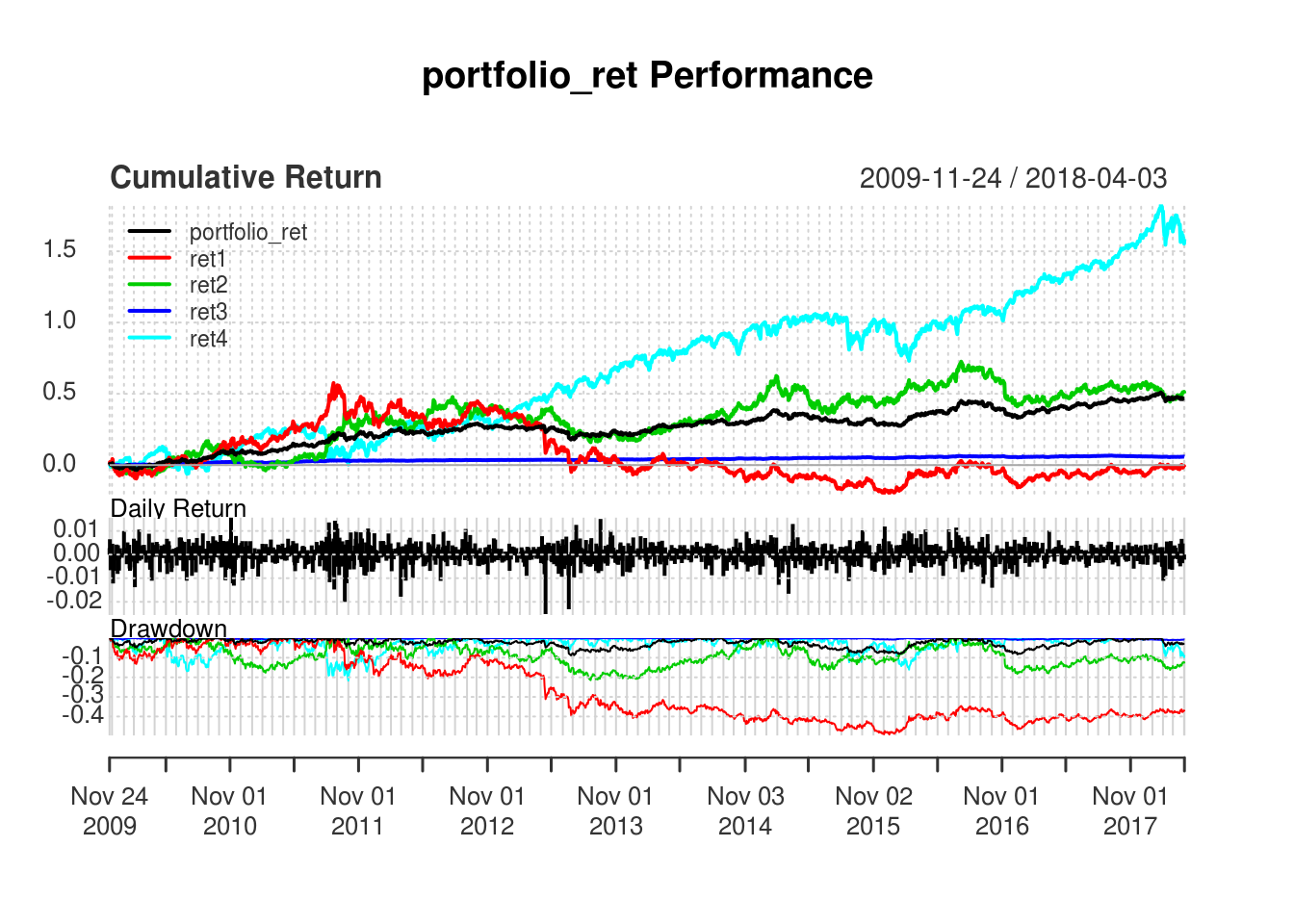
On the annualized returns, it’s not really fantastic. But it still returns a respectable annualized performance of 5% (+ 2% dividends?)
What stands out, however, are the following performance metrics:
- In terms of draw-down, it performed remarkably well relative to a Total US Stock portfolio. It suffered a loss of only 9% as compared to a huge loss of 20 + % in other assets; could be more if full Great Financial Crisis is included.
- On the Sharpe Ratio (annualized returns in excess of risk-free rate per unit of volatility), it’s considerably higher than other assets - albeit lower than Total Stock (in my other analysis with longer time period, it’s considerably higher).
Feel free to adapt or adopt the code. You can easily substitute the stocks based on your preferred asset allocation.
Setting up the analysis.
In this section, I downloaded stock data using quant mod. And merge the time series.
library(quantmod)## Loading required package: xts## Loading required package: zoo##
## Attaching package: 'zoo'## The following objects are masked from 'package:base':
##
## as.Date, as.Date.numeric## Loading required package: TTR## Version 0.4-0 included new data defaults. See ?getSymbols.library(ggplot2)
library(PerformanceAnalytics)##
## Attaching package: 'PerformanceAnalytics'## The following object is masked from 'package:graphics':
##
## legendlibrary(tidyr)
library(dplyr)##
## Attaching package: 'dplyr'## The following objects are masked from 'package:xts':
##
## first, last## The following objects are masked from 'package:stats':
##
## filter, lag## The following objects are masked from 'package:base':
##
## intersect, setdiff, setequal, unionlibrary(tibble)
# Download data-->Fix the ending date for project section
ticker1 = "GLD"
stock1 = getSymbols(ticker1,from="1900-01-01",auto.assign=F)## 'getSymbols' currently uses auto.assign=TRUE by default, but will
## use auto.assign=FALSE in 0.5-0. You will still be able to use
## 'loadSymbols' to automatically load data. getOption("getSymbols.env")
## and getOption("getSymbols.auto.assign") will still be checked for
## alternate defaults.
##
## This message is shown once per session and may be disabled by setting
## options("getSymbols.warning4.0"=FALSE). See ?getSymbols for details.##
## WARNING: There have been significant changes to Yahoo Finance data.
## Please see the Warning section of '?getSymbols.yahoo' for details.
##
## This message is shown once per session and may be disabled by setting
## options("getSymbols.yahoo.warning"=FALSE).names(stock1) = c("open","high","low","close","volume","adj_close")
stock1 = stock1[,6]
ticker2 = "TLT"
stock2 = getSymbols(ticker2,from="1900-01-01",auto.assign=F)
names(stock2) = c("open","high","low","close","volume","adj_close")
stock2 = stock2[,6]
ticker3 = "VGSH"
stock3 = getSymbols(ticker3,from="1900-01-01",auto.assign=F)
names(stock3) = c("open","high","low","close","volume","adj_close")
stock3 = stock3[,6]
ticker4 = "VTI"
stock4 = getSymbols(ticker4,from="1900-01-01",auto.assign=F)
names(stock4) = c("open","high","low","close","volume","adj_close")
stock4 = stock4[,6]
# Merge the time series and subset NA
#These are the various time series
ticker_list = c("stock1","stock2","stock3","stock4")
#read in list. Loop through and assign variable to holder variable. Then assign it to combined list
ticker_all = get(ticker_list[1])
#Merging in the time series
for(i in 2:length(ticker_list)){
ticker_ind = get(ticker_list[i])
ticker_all = merge(ticker_all,ticker_ind)
}
names(ticker_all) = c("stock1","stock2","stock3","stock4")
ticker_all = subset(ticker_all,!is.na(ticker_all$stock1) & !is.na(ticker_all$stock2) & !is.na(ticker_all$stock3) & !is.na(ticker_all$stock4))Running the simulation
Next, I run the simulation - By intialising 25% asset allocation in each of the asset and rebalance at the end of each year. Daily portfolio returns are then obtained throught the ROC function.
#Assign equal weights to each stream of returns
ticker_all = cbind(ticker_all,rowMeans(ticker_all))
ticker_all = subset(ticker_all,!is.na(ticker_all[,4]))
ticker_all = ticker_all[,-ncol(ticker_all)]

#Identify the period of rebalancing. Show the indexes
rebal_index = data.frame(index = endpoints(ticker_all,on="years")[-1])
# endpoints(ticker_all,on="quarters")

#Merge in the indicator into ticker_all--Can't seem to merge. Will do the inefficient loop
# merge(ticker_all,rebal_index, by = "index", all = T)
ticker_all$rebal = NA
for(i in 1:nrow(rebal_index)){
  ticker_all$rebal[rebal_index$index[i]] = 1
}

ticker_all$rebal = ifelse(is.na(ticker_all$rebal),0,ticker_all$rebal)

#Create the returns for each price series
ticker_all$ret1 = ROC(ticker_all[,1])
ticker_all$ret2 = ROC(ticker_all[,2])
ticker_all$ret3 = ROC(ticker_all[,3])
ticker_all$ret4 = ROC(ticker_all[,4])

#Initialise value for each stock series, with a total portfolio value
ticker_all$val1 = NA; ticker_all$val1[1] = 100
ticker_all$val2 = NA; ticker_all$val2[1] = 100
ticker_all$val3 = NA; ticker_all$val3[1] = 100
ticker_all$val4 = NA; ticker_all$val4[1] = 100

ticker_all$portfolio_val = NA
ticker_all$portfolio_val[1] = rowSums(ticker_all[1,which(names(ticker_all) == "val1"):which(names(ticker_all) == "val4")])


#Loop each row and 'compound'. Till it reaches the rebalancing date. Then reset stock value amount in that day. Take the portfolio value in t-1
for(i in 2:nrow(ticker_all)){

  if(as.numeric(ticker_all$rebal[i]) == 0){

  #During non-rebalancing days
  ticker_all$val1[i] = as.numeric(ticker_all$val1[i-1]) * (1 + as.numeric(ticker_all$ret1[i]))
  ticker_all$val2[i] = as.numeric(ticker_all$val2[i-1]) * (1 + as.numeric(ticker_all$ret2[i]))
  ticker_all$val3[i] = as.numeric(ticker_all$val3[i-1]) * (1 + as.numeric(ticker_all$ret3[i]))
  ticker_all$val4[i] = as.numeric(ticker_all$val4[i-1]) * (1 + as.numeric(ticker_all$ret4[i]))

  ticker_all$portfolio_val[i] = rowSums(ticker_all[i,which(names(ticker_all) == "val1"):which(names(ticker_all) == "val4")])

  }else{
  #During re-balancing days
  ticker_all$val1[i] = ticker_all$portfolio_val[i-1] / 4
  ticker_all$val2[i] = ticker_all$portfolio_val[i-1] / 4
  ticker_all$val3[i] = ticker_all$portfolio_val[i-1] / 4
  ticker_all$val4[i] = ticker_all$portfolio_val[i-1] / 4

  ticker_all$portfolio_val[i] = rowSums(ticker_all[i,which(names(ticker_all) == "val1"):which(names(ticker_all) == "val4")])
  }
}

#Generate the daily portfolio returns
ticker_all$portfolio_ret = ROC(ticker_all$portfolio_val)
Portfolio Performance for the entire period
On the annualized returns, it’s not really fantastic. But it still returns a respectable annualized performance of 5% (+ 2% dividends?)
What stands out, however, are the following performance metrics:
- In terms of draw-down, it performed remarkably well relative to a GOLD & Total US Stock portfolio. It suffered a loss of only 9% as compared to a loss of 20+ % in other assets; could’ve be more if full Great Financial Crisis is included (in my post analysis, it could go up to 60% if Great Financial Crisis is included).
- On the Sharpe Ratio (annualized returns in excess of risk-free rate per unit of volatility), it’s considerably higher than other assets - albeit lower than Total Stock (in my other analysis with longer time period, it’s considerably higher).
######################################Study the portfolio returns########################################
#Carry out the portfolio return series
table.Drawdowns(ticker_all$portfolio_ret, top=10)
## From Trough To Depth Length To Trough Recovery
## 1 2012-10-05 2013-06-26 2014-06-19 -0.0882 427 180 247
## 2 2016-07-11 2016-12-15 2017-08-30 -0.0828 289 112 177
## 3 2015-01-26 2016-01-14 2016-06-08 -0.0804 346 246 100
## 4 2009-12-03 2010-02-10 2010-04-14 -0.0471 90 47 43
## 5 2018-01-29 2018-02-08 <NA> -0.0415 46 9 NA
## 6 2011-09-07 2011-09-28 2011-11-03 -0.0409 42 16 26
## 7 2012-02-29 2012-05-16 2012-08-24 -0.0391 125 55 70
## 8 2011-11-08 2011-12-15 2012-01-27 -0.0368 55 27 28
## 9 2010-11-09 2010-11-17 2011-02-28 -0.0317 76 7 69
## 10 2014-09-02 2014-09-17 2014-12-09 -0.0274 70 12 58table.DownsideRisk(merge(ticker_all$portfolio_ret, ticker_all$ret1, ticker_all$ret2, ticker_all$ret3, ticker_all$ret4))## portfolio_ret ret1 ret2 ret3
## Semi Deviation 0.0029 0.0077 0.0065 0.0005
## Gain Deviation 0.0023 0.0066 0.0056 0.0004
## Loss Deviation 0.0028 0.0079 0.0060 0.0004
## Downside Deviation (MAR=210%) 0.0090 0.0128 0.0117 0.0083
## Downside Deviation (Rf=0%) 0.0028 0.0076 0.0064 0.0004
## Downside Deviation (0%) 0.0028 0.0076 0.0064 0.0004
## Maximum Drawdown 0.0882 0.4922 0.2147 0.0106
## Historical VaR (95%) -0.0062 -0.0169 -0.0146 -0.0010
## Historical ES (95%) -0.0090 -0.0253 -0.0193 -0.0014
## Modified VaR (95%) -0.0064 -0.0177 -0.0146 -0.0010
## Modified ES (95%) -0.0108 -0.0342 -0.0210 -0.0015
## ret4
## Semi Deviation 0.0071
## Gain Deviation 0.0062
## Loss Deviation 0.0077
## Downside Deviation (MAR=210%) 0.0119
## Downside Deviation (Rf=0%) 0.0069
## Downside Deviation (0%) 0.0069
## Maximum Drawdown 0.2169
## Historical VaR (95%) -0.0158
## Historical ES (95%) -0.0237
## Modified VaR (95%) -0.0158
## Modified ES (95%) -0.0294table.AnnualizedReturns(merge(ticker_all$portfolio_ret, ticker_all$ret1, ticker_all$ret2, ticker_all$ret3, ticker_all$ret4))## portfolio_ret ret1 ret2 ret3 ret4
## Annualized Return 0.0469 -0.0017 0.0500 0.0069 0.1206
## Annualized Std Dev 0.0611 0.1651 0.1427 0.0101 0.1519
## Annualized Sharpe (Rf=0%) 0.7674 -0.0103 0.3503 0.6756 0.7937charts.PerformanceSummary(merge(ticker_all$portfolio_ret, ticker_all$ret1, ticker_all$ret2, ticker_all$ret3, ticker_all$ret4))
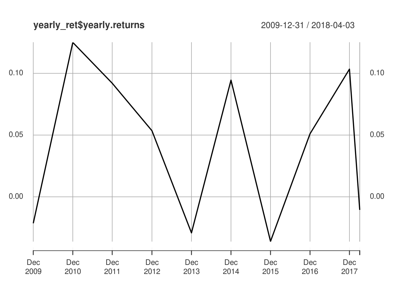
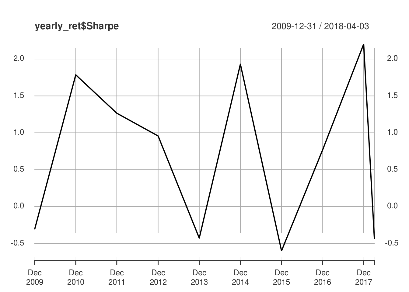
Yearly Portfolio Performance
I also tabulated the yearly metrics of the portfolio to give a sense of the performance over years.
#####################################Study the annualized portfolio returns series#######################
#Use the rebal-indicator. Loop through the chunks
# https://www.quantmod.com/documentation/periodReturn.html
# https://rpubs.com/mohammadshadan/288218
# yearly_ret = periodReturn(ticker_all$portfolio_val
#              ,period='yearly',subset='2004::')  # returns years 2003 to present

yearly_ret = periodReturn(ticker_all$portfolio_val
                          ,period='yearly')  # returns years 2003 to present

#Inefficient way to calulate standard deviation. If it've time, I will probably optimize this
split_val = split(ticker_all$portfolio_ret, f = "years")
yearly_ret$annual_sd = sapply(X = split_val, FUN = StdDev) * sqrt(252)


getSymbols('DGS3MO',src = 'FRED')
## [1] "DGS3MO"rf = DGS3MO; rm(DGS3MO)
rf = rf["2009/2018"]
split_val_rf = split(rf$DGS3MO, f = "years")
yearly_ret$annual_rf = sapply(X = split_val_rf, FUN = mean, na.rm = T)/100
yearly_ret$Sharpe = (yearly_ret$yearly.returns - yearly_ret$annual_rf)/yearly_ret$annual_sd
yearly_ret## yearly.returns annual_sd annual_rf Sharpe
## 2009-12-31 -0.02143548 0.07391424 0.0015092000 -0.3104230
## 2010-12-31 0.12503869 0.06925292 0.0013844622 1.7855452
## 2011-12-30 0.09201080 0.07228724 0.0005284000 1.2655400
## 2012-12-31 0.05353343 0.05504939 0.0008760000 0.9565489
## 2013-12-31 -0.02919578 0.06965068 0.0005708000 -0.4273696
## 2014-12-31 0.09449067 0.04879063 0.0003272000 1.9299499
## 2015-12-31 -0.03608942 0.06101808 0.0005250996 -0.6000601
## 2016-12-30 0.05106338 0.06221028 0.0031936000 0.7694834
## 2017-12-29 0.10340429 0.04264321 0.0094896000 2.2023362
## 2018-04-03 -0.01057814 0.06051025 0.0158516129 -0.4367815plot(yearly_ret$yearly.returns)
plot(yearly_ret$Sharpe)