Simulating product failures
I’m inspired by this post here (http://www.programmingr.com/examples/neat-tricks/sample-r-function/rexp/). And decided to expand on the example.
Say you are an owner of a computer store and you would like to estimate the frequency of warranty repairs - and the ensuing costs.
Here’s the scenario with the accompanying assumptions
- Each computer is expected to last an average of 7 years
- You only sell 1000 computers at the start of each year
- You sell computer from 2019 to 2025
First, I simulate an exponential distribution of 1000 points for 7 years; and place a time index of 2019 to 2025
set.seed(1)
library(tidyr)

sim_repair_time = mapply(rexp, rep(1000, 7), rep(1/7, 7))
sim_repair_time = data.frame(sim_repair_time)
names(sim_repair_time) = paste0("Y", 2019:2025)
sim_repair_time$comp_index = 1:nrow(sim_repair_time)
head(sim_repair_time)
## Y2019 Y2020 Y2021 Y2022 Y2023 Y2024 Y2025
## 1 5.2862728 7.0456022 4.4584814 2.987471 2.4983623 1.155475 3.526856
## 2 8.2714995 0.3831851 21.3583423 16.976357 0.6371918 19.870135 8.339298
## 3 1.0199471 6.1577002 24.7270286 7.184722 13.6686444 2.692336 1.531733
## 4 0.9785668 2.0554758 4.0556961 11.680879 3.4047724 8.547126 4.098845
## 5 3.0524804 1.3899782 0.8014122 7.394160 10.8930823 1.088804 8.679067
## 6 20.2647798 1.1392965 8.5595344 3.423599 5.0281127 8.178582 15.854250
## comp_index
## 1 1
## 2 2
## 3 3
## 4 4
## 5 5
## 6 6Then, I - in dplyr lingo - gather the dataset (convert to long form)
sim_repair_time = sim_repair_time %>% gather(key = year,
                                     value = spoilt_years_later,
                                    -comp_index)
sim_repair_time$year = gsub("Y", "", sim_repair_time$year)

head(sim_repair_time, 50)
## comp_index year spoilt_years_later
## 1 1 2019 5.2862728
## 2 2 2019 8.2714995
## 3 3 2019 1.0199471
## 4 4 2019 0.9785668
## 5 5 2019 3.0524804
## 6 6 2019 20.2647798
## 7 7 2019 8.6069344
## 8 8 2019 3.7777799
## 9 9 2019 6.6959725
## 10 10 2019 1.0293219
## 11 11 2019 9.7351459
## 12 12 2019 5.3342090
## 13 13 2019 8.6632249
## 14 14 2019 30.9675395
## 15 15 2019 7.3818022
## 16 16 2019 7.2467076
## 17 17 2019 13.1322462
## 18 18 2019 4.5832265
## 19 19 2019 2.3585343
## 20 20 2019 4.1193581
## 21 21 2019 16.5516068
## 22 22 2019 4.4932481
## 23 23 2019 2.0588427
## 24 24 2019 3.9610587
## 25 25 2019 0.7425084
## 26 26 2019 0.4160741
## 27 27 2019 4.0509872
## 28 28 2019 27.7125300
## 29 29 2019 8.2131847
## 30 30 2019 6.9776907
## 31 31 2019 10.0469974
## 32 32 2019 0.2608797
## 33 33 2019 2.2680711
## 34 34 2019 9.2432755
## 35 35 2019 1.4245725
## 36 36 2019 7.1590811
## 37 37 2019 2.1121865
## 38 38 2019 5.0765001
## 39 39 2019 5.2607988
## 40 40 2019 1.6451922
## 41 41 2019 7.5591680
## 42 42 2019 7.1977283
## 43 43 2019 9.0458315
## 44 44 2019 8.7717375
## 45 45 2019 3.8824898
## 46 46 2019 2.1089810
## 47 47 2019 9.0518726
## 48 48 2019 6.9618905
## 49 49 2019 3.5992201
## 50 50 2019 14.0548268Lastly, I add the time taken for each computer to break down to the year for which the computer is bought.
#sim_repair_time$spoilt_years_later = round(sim_repair_time$spoilt_years_later, 0)
sim_repair_time$year_spoilt = sim_repair_time$spoilt_years_later + as.numeric(sim_repair_time$year)
Here is the distribution of years taken that a computer will break down.
hist(sim_repair_time$spoilt_years_later)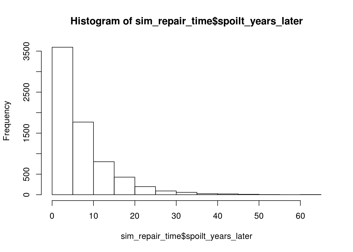
And here is the distribution of the years that the computer will break down.
hist(sim_repair_time$year_spoilt)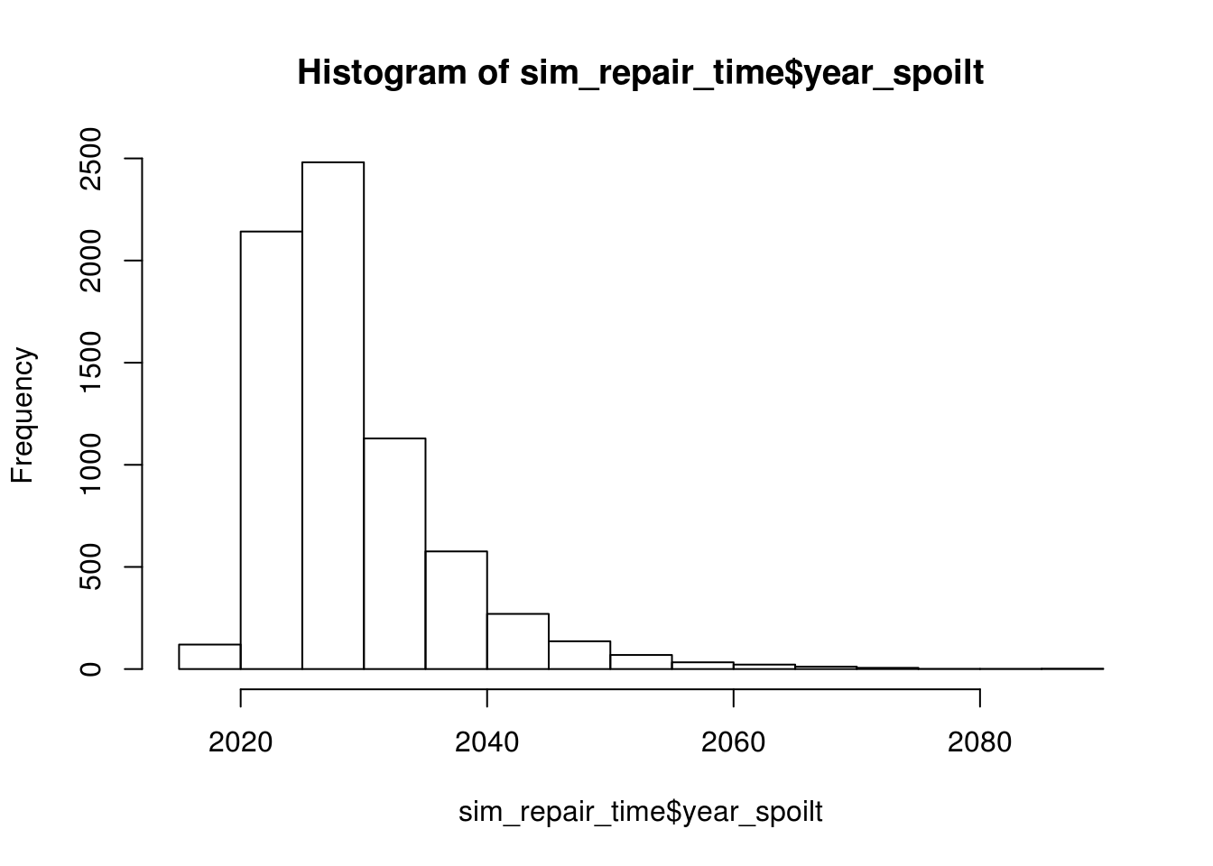
Explaining exponential distribution from first principle
If you are keen from the first principle perspective,
\[f(x) = {\lambda}e^{-\lambda x} \]
To understand pdf function here. It’s pretty simple. If you run the simulator 1000 times with mean = 7 (lambda = 1/7), and you plot the distribution, it’s mostly likely to be front-loaded.
If you fit a series of values x - N to the above function, it will be pretty similar to simulated series of values.
And if you do a mean of the simulated data, it will return close to the mean of 7
data = rexp(1000, 1/7)
hist(data)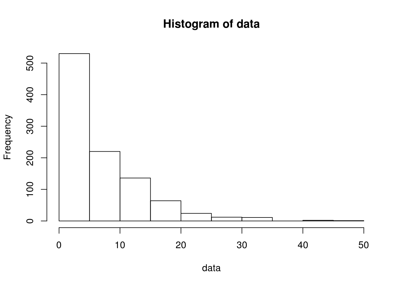
mean(data)## [1] 6.775649I hope this simple example here is useful!