Decomposing a Position Into Exchange Rate and Non Exchange Rate Effects
If you are someone with a stake in foreign positions, this package I wrote here may be a useful tool to help you understand the impact of foreign currency on your positions. For instance,
- If you are an investor, you may use it to analyze impact of exchange rate on your investment positions.
- If you are in the treasury department, you may wish to analyze the impact of exchange rates on your bonds.
- If you are in the finance department, you could analyze the exchange rate impact on your foreign revenue.
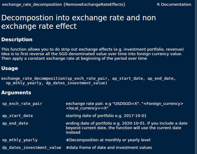
To start using this package, you may first install the devtools package and execute the following command. install_github(“jironghuang/RemoveExchangeRateEffects”). The R documentation is as follows,

You may follow the 2 examples to better understand how this package works.
Example 1
In summary, what the example does below is to decompose 1 instrument position in SGD (column value) - from the perspective of someone staying in Singapore - into local static value (i.e if I keep the exchange rate constant at the start of the period) and the residual exchange rate impact.
If you look at the value at the end of the period (Oct 2018), you would notice that the value in SGD fell from 331 to 261. From the perspective of a Singaporean local - through this package - we can understand that the appreciation in USD negate the fall in value by 4 SGD.
If you are an economist, you could have considered the exchange rate elasticities. But let’s ignore that for now.
Quick example 1 in R codes (decomposing a single instrument)
library(devtools)
install_github("jironghuang/RemoveExchangeRateEffects")
library(RemoveExchangeRateEffects)

sp_exch_rate_pair = "USDSGD=X"  #exchange rate pair. e.g "USDSGD=X". "<Foreign_currency><local_currency>=X"

ap_start_date <- as.Date("2017-10-01")  #starting date of portfolio e.g. 2017-10-01
ap_end_date <- as.Date("2020-10-01") #ending date of portfolio e.g. 2020-10-01. If you include a date beyond current date, the function will use the current date instead
np_mthly_yearly = "monthly"  #alternatively this could be "yearly""

data(eg_dat) #example dataset that I included in this package
dp_dates_investment_value = instrument
o_exchRate_effect <- exchange_rate_decomposition(sp_exch_rate_pair, ap_start_date, ap_end_date, np_mthly_yearly, dp_dates_investment_value)
o_exchRate_effect$get_portfolio()

    value_in_sgd exchange_rate fgn_value local_static_value exch_rate_impact
Oct 2017 331.53   1.36010  243.7541           331.5300        0.0000000
Nov 2017 308.85   1.34670  229.3384           311.9231       -3.0731344
Dec 2017 311.35   1.33780  232.7328           316.5399       -5.1899425
Jan 2018 354.31   1.31168  270.1192           367.3892      -13.0791734
Feb 2018 343.06   1.32433  259.0442           352.3260       -9.2660108
Mar 2018 266.13   1.31090  203.0132           276.1183       -9.9882495
Apr 2018 293.90   1.32577  221.6825           301.5104       -7.6103599
May 2018 284.73   1.33850  212.7232           289.3248       -4.5948212
Jun 2018 342.95   1.36830  250.6395           340.8948        2.0552438
Jul 2018 298.14   1.36140  218.9952           297.8553        0.2846937
Aug 2018 301.66   1.36700  220.6730           300.1374        1.5226438
Sep 2018 264.77   1.36732  193.6416           263.3719        1.3980921
Oct 2018 260.95   1.38061  189.0107           257.0734        3.8766087

o_exchRate_effect$get_diff_portfolio_value()
[1] 3.8766087
Example 2
The second example builds upon the first. I’ve expanded the previous function to decompose multiple instruments at once.
get_full_decomposition() returns a list of data frames with the decompositions.
But before you implement the function above, you would have to add the information via the mutator functions as shown in the example below (the functions with the prefix set)
Quick example 2 in R codes (Decomposing multiple instruments at 1 time)
data(eg_dat)

er = c("USDSGD=X", "GBPSGD=X")
start_date = c("2017-10-01", "2017-10-01")
end_date = c("2020-10-01", "2020-10-01")
freq = c("monthly", "monthly")
dat = list(eg_dat, eg_dat)


o_exchRate_effect <- multiple_exchange_rate_decomposition(2)
o_exchRate_effect$set_sa_exch_rate_pair(er) #adding an array of exchange rate pairs
o_exchRate_effect$set_sa_start_date(start_date) #adding an array of starting dates
o_exchRate_effect$set_sa_end_date(end_date) #adding an array of ending dates
o_exchRate_effect$set_sa_mthly_yearly(freq) #adding an array of "monthly" or "yearly" option
o_exchRate_effect$set_dl_dates_investment_value(dat) #adding list of data frames
o_exchRate_effect$get_full_decomposition()  #carry out decomposition and obtain a list of data frames

[[1]]
          value exchange_rate fgn_value local_static_value exch_rate_impact
Oct 2017 331.53       1.36010  243.7541           331.5300        0.0000000
Nov 2017 308.85       1.34670  229.3384           311.9231       -3.0731344
Dec 2017 311.35       1.33780  232.7328           316.5399       -5.1899425
Jan 2018 354.31       1.31168  270.1192           367.3892      -13.0791734
Feb 2018 343.06       1.32433  259.0442           352.3260       -9.2660108
Mar 2018 266.13       1.31090  203.0132           276.1183       -9.9882495
Apr 2018 293.90       1.32577  221.6825           301.5104       -7.6103599
May 2018 284.73       1.33850  212.7232           289.3248       -4.5948212
Jun 2018 342.95       1.36830  250.6395           340.8948        2.0552438
Jul 2018 298.14       1.36140  218.9952           297.8553        0.2846937
Aug 2018 301.66       1.36700  220.6730           300.1374        1.5226438
Sep 2018 264.77       1.36732  193.6416           263.3719        1.3980921
Oct 2018 260.95       1.38061  189.0107           257.0734        3.8766087

[[2]]
          value exchange_rate fgn_value local_static_value exch_rate_impact
Oct 2017 331.53       1.79703  184.4877           331.5300        0.0000000
Nov 2017 308.85       1.80690  170.9281           307.1629        1.6870605
Dec 2017 311.35       1.79812  173.1531           311.1613        0.1887369
Jan 2018 354.31       1.85680  190.8175           342.9048       11.4051640
Feb 2018 343.06       1.84162  186.2816           334.7537        8.3062984
Mar 2018 266.13       1.83911  144.7059           260.0408        6.0892228
Apr 2018 293.90       1.82588  160.9635           289.2562        4.6437963
May 2018 284.73       1.77878  160.0704           287.6513       -2.9212846
Jun 2018 342.95       1.78907  191.6918           344.4759       -1.5258666
Jul 2018 298.14       1.78638  166.8962           299.9175       -1.7774444
Aug 2018 301.66       1.77860  169.6053           304.7858       -3.1258259
Sep 2018 264.77       1.78285  148.5094           266.8759       -2.1058633
Oct 2018 260.95       1.76900  147.5127           265.0848       -4.1347817