Analysis of Market Cap to GDP
Warren Buffett, the world’s greatest investor once remarked that Country’s Total Market Capitalization to GDP ratio is a good indicator to measure the ‘temperature’ of the market. My wild guess is - he draws his inspiration from P/E ratio where price correspondes to the Total Market Cap and GDP to Earnings.
Key points
- By historical standards, the Market Cap to GDP ratios are currently way above the average, 5-year and 10-year averages
- This may spell some bad news in the near term. What goes up would eventually come down. Caveat: I noticed that the ratio is trending upwards over time. Perhaps I could account for that using a time-trend in the future.
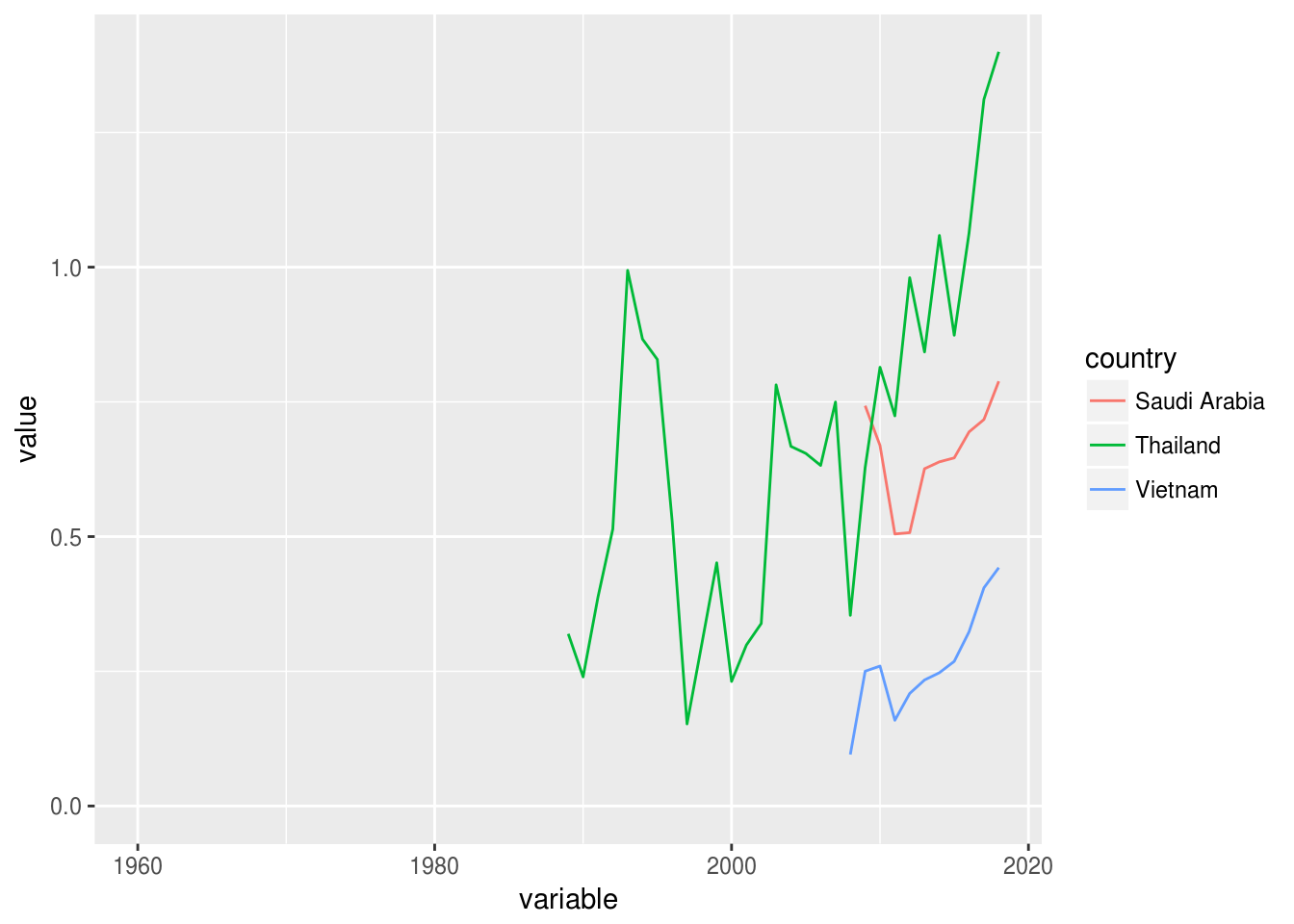
- Of the countries that are ‘heated’, Belgium, France, Saudi Arabia, Thailand and Vietnam are at all-time high. Shorting could be an option but please conduct additional analysis before deciding on a position.
- P/E ratios of these ETFs could be used to supplement this analysis. Unfortunately I don’t have a set of readily ‘analyzable’ data.
- Alternatively, we could rely on the % from 52 week high as an indicator (wrote an article on this in my Linkedin articles section (https://www.linkedin.com/pulse/investment-compass-our-volatile-times-jirong-huang/); also developed an ugly Shiny real-time dashboard but I’ll only share it when I’m pleased with my GUI design).
Future developments
I’ve plans to convert this to an interactive real-time dashboard hosted in the cloud. But this really depends on my spare capacity.
Disclosure
On 2 April 2018, I initiated a small short position on South Africa (EZA) at 67.58 because I believe it’s really over-heated (based on P/E and this analysis here).
Setting up analysis and loading in necessary libraries
#Macro analysis on Mkt cap to GDP
#Do trailing 5 year averages
#Maybe better t
#Rebase to 2016 using GFP growth figures for key countries

library("WDI")
## Loading required package: RJSONIOlibrary("reshape2")
library("rvest")## Loading required package: xml2library("ggplot2")
rm(list = ls())
# hk_ind = (3193235.54 * 1000000)/(320.9 * 1000000000)
setwd("/home/jirong/Dropbox/macro analysis")Extracting GDP and Country’s Total Market Capitalization via its API (Before 2017)
I first extract the Countries’ Market Cap and GDP data form World Bank’s API. But the current dataset is only updated till 2016 in its database.
##################################Trying out world bank API########################
#Market cap data
mkt_cap = WDI(country = "all", indicator = "CM.MKT.LCAP.CD",
    start = 1900, end = 2018, extra = FALSE, cache = NULL)


names(mkt_cap)[which(names(mkt_cap) == "CM.MKT.LCAP.CD")] = "value"

#Cast the dataframes
mkt_cap_wide = dcast(mkt_cap,country ~ year,na.rm = T)


#GDP data-->NY.GDP.MKTP.CD
gdp = WDI(country = "all", indicator = "NY.GDP.MKTP.CD",
              start = 1900, end = 2018, extra = FALSE, cache = NULL)

names(gdp)[which(names(gdp) == "NY.GDP.MKTP.CD")] = "value"

#Cast the dataframes
gdp_wide = dcast(gdp,country ~ year,na.rm = T)

#For a start-->Scrape the data from wikipedia-->Port it to a google sheet-->To 'project' the 2017 GDP growth rates
#https://en.wikipedia.org/wiki/List_of_countries_by_real_GDP_growth_rate
Extracting 2017 GDP Growth Rate from Wikipedia Page
Since WB’s APi lack 2017 data, I had to crawl the 2017 GDP growth rate from Wikipedia to extapolate the 2017 GDP.
There may be some issues on using real and nominal GDP growth rates but I’ll choose to ignore that for now.
For simplicity, I assume 2018’s GDP to be same as 2017. I could have used the projected 2018 GDP from World Bank or IMF but those data are not readily available (for crawling or through API). Or maybe I’m too plain lazy!
url <- "https://en.wikipedia.org/wiki/List_of_countries_by_real_GDP_growth_rate#cite_note-1"

webpage = read_html(url)
tbls <- html_nodes(webpage, "table")
tbls_ls <- webpage %>%
  html_nodes("table") %>%
  .[1:4] %>%
  html_table(fill = TRUE)

gdp_growth = tbls_ls[[1]]  #GDP real growth rates
names(gdp_growth) = c("rank","country","gdp_rate")

#Remove all []
for(i in 2:ncol(gdp_growth)){
  gdp_growth[,i] = gsub("\\[.*\\]","",gdp_growth[,i])
}
gdp_growth$gdp_rate = as.numeric(gdp_growth$gdp_rate)

#Merge in to the data frame
gdp_wide = merge(gdp_wide,gdp_growth, by = "country", all.x = T)
gdp_wide = gdp_wide[!duplicated(gdp_wide$country),]

gdp_wide$`2017` = gdp_wide$`2016` * (1+ gdp_wide$gdp_rate/100)

#removing unnecssary names
gdp_wide = gdp_wide[,-which(names(gdp_wide) == "rank")]
gdp_wide = gdp_wide[,-which(names(gdp_wide) == "gdp_rate")]

#Assume 2018 GDP to be same as 2017
gdp_wide$`2018` = gdp_wide$`2017`
Extracting 2017-2018 Stock Prices
To obtain the 2017 and latest Countries’ Market Captialization, I developed an ingenious way!
I first mapped each country to an ETF in New York Stock Exchange at the end of this section.
Next, I accessed Google Finance API via a script “match_WB_US_ticker.R”. This is a fairly complicated script that I choose not to show here - pls PM me if you wish to have it.
Then I compute the ETF’s returns from Jan 2017 (to end 2017 and current price) and mapped the growth rates on end 2016 WB market capitalization data. This allows me to impute the country’s market capitalization in 2017 and the updated (1 April 2018) Country’s Market Capitalization.
- wb_ticker$ticker = NA
- wb_ticker\(ticker[which(wb_ticker\)country == “Arab World”)] = “MES”
- wb_ticker\(ticker[which(wb_ticker\)country == “Argentina”)] = “ARGT”
- wb_ticker\(ticker[which(wb_ticker\)country == “Australia”)] = “EWA”
- wb_ticker\(ticker[which(wb_ticker\)country == “Austria”)] = “EWO”
- wb_ticker\(ticker[which(wb_ticker\)country == “Belgium”)] = “EWK”
- wb_ticker\(ticker[which(wb_ticker\)country == “Brazil”)] = “EWZ”
- wb_ticker\(ticker[which(wb_ticker\)country == “Canada”)] = “EWC”
- wb_ticker\(ticker[which(wb_ticker\)country == “Chile”)] = “ECH”
- wb_ticker\(ticker[which(wb_ticker\)country == “China”)] = “MCHI”
- wb_ticker\(ticker[which(wb_ticker\)country == “Colombia”)] = “ICOL”
- wb_ticker\(ticker[which(wb_ticker\)country == “Denmark”)] = “EDEN” #Something wrong with this
- wb_ticker\(ticker[which(wb_ticker\)country == “Euro area”)] = “IEV”
- wb_ticker\(ticker[which(wb_ticker\)country == “European Union”)] = “EZU”
- wb_ticker\(ticker[which(wb_ticker\)country == “France”)] = “EWQ”
- wb_ticker\(ticker[which(wb_ticker\)country == “Germany”)] = “EWG”
- wb_ticker\(ticker[which(wb_ticker\)country == “Greece”)] = “GREK”
- wb_ticker\(ticker[which(wb_ticker\)country == “Hong Kong SAR, China”)] = “EWH”
- wb_ticker\(ticker[which(wb_ticker\)country == “India”)] = “INDA”
- wb_ticker\(ticker[which(wb_ticker\)country == “Indonesia”)] = “EIDO”
- wb_ticker\(ticker[which(wb_ticker\)country == “Ireland”)] = “EIRL”
- wb_ticker\(ticker[which(wb_ticker\)country == “Israel”)] = “EIS”
- wb_ticker\(ticker[which(wb_ticker\)country == “Italy”)] = “EWI”
- wb_ticker\(ticker[which(wb_ticker\)country == “Japan”)] = “EWJ”
- wb_ticker\(ticker[which(wb_ticker\)country == “Ireland”)] = “EIRL”
- wb_ticker\(ticker[which(wb_ticker\)country == “Korea, Rep.”)] = “EWY”
- wb_ticker\(ticker[which(wb_ticker\)country == “Malaysia”)] = “EWM”
- wb_ticker\(ticker[which(wb_ticker\)country == “Ireland”)] = “EIRL”
- wb_ticker\(ticker[which(wb_ticker\)country == “Meixco”)] = “EWW”
- wb_ticker\(ticker[which(wb_ticker\)country == “Netherlands”)] = “EWN”
- wb_ticker\(ticker[which(wb_ticker\)country == “New Zealand”)] = “ENZL”
- wb_ticker\(ticker[which(wb_ticker\)country == “Nigeria”)] = “NGE”
- wb_ticker\(ticker[which(wb_ticker\)country == “Netherlands”)] = “EWN”
- wb_ticker\(ticker[which(wb_ticker\)country == “Netherlands”)] = “EWN”
- wb_ticker\(ticker[which(wb_ticker\)country == “Norway”)] = “ENOR”
- wb_ticker\(ticker[which(wb_ticker\)country == “Peru”)] = “EPU”
- wb_ticker\(ticker[which(wb_ticker\)country == “Philippines”)] = “EPHE”
- wb_ticker\(ticker[which(wb_ticker\)country == “Poland”)] = “EPOL”
- wb_ticker\(ticker[which(wb_ticker\)country == “Portugal”)] = “PGAL”
- wb_ticker\(ticker[which(wb_ticker\)country == “Qatar”)] = “QAT”
- wb_ticker\(ticker[which(wb_ticker\)country == “Portugal”)] = “PGAL”
- wb_ticker\(ticker[which(wb_ticker\)country == “Russian Federation”)] = “ERUS”
- wb_ticker\(ticker[which(wb_ticker\)country == “Saudi Arabia”)] = “KSA”
- wb_ticker\(ticker[which(wb_ticker\)country == “Singapore”)] = “EWS”
- wb_ticker\(ticker[which(wb_ticker\)country == “South Africa”)] = “EZA”
- wb_ticker\(ticker[which(wb_ticker\)country == “Spain”)] = “EWP”
- wb_ticker\(ticker[which(wb_ticker\)country == “Sweden”)] = “EWD”
- wb_ticker\(ticker[which(wb_ticker\)country == “Switzerland”)] = “EWL”
- wb_ticker\(ticker[which(wb_ticker\)country == “Thailand”)] = “THD”
- wb_ticker\(ticker[which(wb_ticker\)country == “Turkey”)] = “TUR”
- wb_ticker\(ticker[which(wb_ticker\)country == “United Kingdom”)] = “EWU”
- wb_ticker\(ticker[which(wb_ticker\)country == “United States”)] = “VTI”
- wb_ticker\(ticker[which(wb_ticker\)country == “Vietnam”)] = “VNM”
- wb_ticker\(ticker[which(wb_ticker\)country == “World”)] = “VT”
#For each country, assign a ticker symbol from NYSE
#Store the end 2016 price and the most updated price now. Then pluck the growth rate on the market cap
source("match_WB_US_ticker.R")
## Loading required package: xts## Loading required package: zoo##
## Attaching package: 'zoo'## The following objects are masked from 'package:base':
##
## as.Date, as.Date.numeric## Loading required package: TTR## Version 0.4-0 included new data defaults. See ?getSymbols.## 'getSymbols' currently uses auto.assign=TRUE by default, but will
## use auto.assign=FALSE in 0.5-0. You will still be able to use
## 'loadSymbols' to automatically load data. getOption("getSymbols.env")
## and getOption("getSymbols.auto.assign") will still be checked for
## alternate defaults.
##
## This message is shown once per session and may be disabled by setting
## options("getSymbols.warning4.0"=FALSE). See ?getSymbols for details.##
## WARNING: There have been significant changes to Yahoo Finance data.
## Please see the Warning section of '?getSymbols.yahoo' for details.
##
## This message is shown once per session and may be disabled by setting
## options("getSymbols.yahoo.warning"=FALSE).## Warning: MES download failed; trying again.
## Warning: MES download failed; trying again.mkt_cap_wide = merge(mkt_cap_wide,wb_ticker, by = "country", all.x = T)
mkt_cap_wide$`2017` = mkt_cap_wide$`2016` * (1+mkt_cap_wide$returns_17)
mkt_cap_wide$`2018` = mkt_cap_wide$`2016` * (1+mkt_cap_wide$returns)
mkt_cap_wide = mkt_cap_wide[,-which(names(mkt_cap_wide) == "returns")]
mkt_cap_wide = mkt_cap_wide[,-which(names(mkt_cap_wide) == "returns_17")]Calculating Market Cap to GDP Ratio
Here, I simply divide the countries’ total market capitalization over their GDPs
#Plot the market cap to growth rates
#Check if names are the same
nrow(gdp_wide) == sum(mkt_cap_wide$country == gdp_wide$country)
## [1] TRUEmkt_cap_gdp = mkt_cap_wide
mkt_cap_gdp[,2:ncol(mkt_cap_gdp)] = mkt_cap_wide[,2:ncol(mkt_cap_wide)] / gdp_wide[,2:ncol(gdp_wide)]
mkt_cap_gdp = subset(mkt_cap_gdp,!is.na(mkt_cap_gdp$`2018`))Finding current level relative to averages and all-time high
To understand if the current level is high, I derive the historical average, 5-year average and 10-year averages.
#Use apply function to find the average, 5 year average, 10 year average, 20 year average
#Find historical average
avg = apply(mkt_cap_gdp[,c(-1,-which(names(mkt_cap_gdp) == "2018"))],1,mean,na.rm = T)

#Find 5-year average
avg_5 = apply(mkt_cap_gdp[,-c(1,which(names(mkt_cap_gdp) == "2018"),
                              which(names(mkt_cap_gdp) == "1960"):
                              which(names(mkt_cap_gdp) == "2012"))],
                              1,mean,na.rm = T)

#Find 10-year average
avg_10 = apply(mkt_cap_gdp[,-c(1,which(names(mkt_cap_gdp) == "2018"),
                               which(names(mkt_cap_gdp) == "1960"):
                               which(names(mkt_cap_gdp) == "2007"))],1,mean,na.rm = T)

#Find max
max_ratio = apply(mkt_cap_gdp[,c(-1,-which(names(mkt_cap_gdp) == "2018"))],1,max,na.rm = T)

#Find min
min_ratio = apply(mkt_cap_gdp[,c(-1,-which(names(mkt_cap_gdp) == "2018"))],1,min,na.rm = T)

#Form a new data frame
avg_ratios = data.frame(country = mkt_cap_gdp$country, avg = avg, avg_5 = avg_5, avg_10 = avg_10)


#See if undervalued or overvalued
mkt_cap_gdp$more_avg = ifelse(mkt_cap_gdp$`2018` > avg_ratios$avg,1,0)
mkt_cap_gdp$more_avg_5 = ifelse(mkt_cap_gdp$`2018` > avg_ratios$avg_5,1,0)
mkt_cap_gdp$more_avg_10 = ifelse(mkt_cap_gdp$`2018` > avg_ratios$avg_10,1,0)

mkt_cap_gdp$less_avg = ifelse(mkt_cap_gdp$`2018` < avg_ratios$avg,1,0)
mkt_cap_gdp$less_avg_5 = ifelse(mkt_cap_gdp$`2018` < avg_ratios$avg_5,1,0)
mkt_cap_gdp$less_avg_10 = ifelse(mkt_cap_gdp$`2018` < avg_ratios$avg_10,1,0)

#See if it's at all time high
mkt_cap_gdp$all_time_high = ifelse(mkt_cap_gdp$`2018` > max_ratio,1,0)

#See if it's at all time low
mkt_cap_gdp$all_time_low = ifelse(mkt_cap_gdp$`2018` < min_ratio,1,0)
Displaying the tabular data
library(knitr)
library(kableExtra)

###################################Subset data frame to flash it out as table############################
#Subset country and indicators
dat = subset(mkt_cap_gdp,select = c("country","2018","all_time_high","all_time_low" ,"more_avg",
                                    "more_avg_5","more_avg_10","less_avg","less_avg_5","less_avg_10"))


dat$avg = avg
dat$avg_5 = avg_5
dat$avg_10 = avg_10
dat$max_ratio = max_ratio
dat$min_ratio = min_ratio

dat = subset(dat,select = c( "country","2018","avg","avg_5", "avg_10", "max_ratio", "min_ratio",
                             "all_time_high", "all_time_low", "more_avg","more_avg_5","more_avg_10","less_avg","less_avg_5",
                             "less_avg_10"   ))

kable(dat, caption = "Summarized data") | country | 2018 | avg | avg_5 | avg_10 | max_ratio | min_ratio | all_time_high | all_time_low | more_avg | more_avg_5 | more_avg_10 | less_avg | less_avg_5 | less_avg_10 | |
|---|---|---|---|---|---|---|---|---|---|---|---|---|---|---|---|
| 9 | Argentina | 0.1702098 | 0.1096417 | 0.1185503 | 0.1136155 | 0.2742805 | 0.0115399 | 0 | 0 | 1 | 1 | 1 | 0 | 0 | 0 |
| 12 | Australia | 1.0827862 | 0.7849408 | 0.9698462 | 0.9894222 | 1.5206944 | 0.2141006 | 0 | 0 | 1 | 1 | 1 | 0 | 0 | 0 |
| 13 | Austria | 0.4516026 | 0.1747203 | 0.2996147 | 0.2738809 | 0.6083190 | 0.0119132 | 0 | 0 | 1 | 1 | 1 | 0 | 0 | 0 |
| 20 | Belgium | 0.9554392 | 0.4576344 | 0.8203120 | 0.6552541 | 0.9667037 | 0.0786858 | 0 | 0 | 1 | 1 | 1 | 0 | 0 | 0 |
| 28 | Brazil | 0.5376609 | 0.4864667 | 0.3885210 | 0.4761217 | 0.9804070 | 0.2495489 | 0 | 0 | 1 | 1 | 1 | 0 | 0 | 0 |
| 37 | Canada | 1.3066000 | 1.0294271 | 1.2141208 | 1.1505540 | 2.1421613 | 0.2730157 | 0 | 0 | 1 | 1 | 1 | 0 | 0 | 0 |
| 44 | Chile | 1.2000244 | 0.9780697 | 0.9359206 | 1.0560277 | 1.5640281 | 0.6357907 | 0 | 0 | 1 | 1 | 1 | 0 | 0 | 0 |
| 45 | China | 0.9207308 | 0.5541939 | 0.6586526 | 0.5922091 | 1.2608774 | 0.1757910 | 0 | 0 | 1 | 1 | 1 | 0 | 0 | 0 |
| 46 | Colombia | 0.4135887 | 0.4740204 | 0.3968742 | 0.4980473 | 0.7264409 | 0.2948531 | 0 | 0 | 0 | 1 | 0 | 1 | 0 | 1 |
| 81 | France | 1.0820485 | 0.4627055 | 0.8749564 | 0.7540257 | 1.0904311 | 0.0505182 | 0 | 0 | 1 | 1 | 1 | 0 | 0 | 0 |
| 86 | Germany | 0.5758399 | 0.3124133 | 0.5134009 | 0.4394087 | 0.6514221 | 0.0757537 | 0 | 0 | 1 | 1 | 1 | 0 | 0 | 0 |
| 89 | Greece | 0.2239557 | 0.3887054 | 0.2454864 | 0.2349021 | 0.8319075 | 0.1173702 | 0 | 0 | 0 | 0 | 0 | 1 | 1 | 1 |
| 109 | India | 0.8106731 | 0.7686539 | 0.7322268 | 0.7421990 | 1.5145139 | 0.4654705 | 0 | 0 | 1 | 1 | 1 | 0 | 0 | 0 |
| 110 | Indonesia | 0.4807856 | 0.3316202 | 0.4457203 | 0.4165210 | 0.5079426 | 0.1264619 | 0 | 0 | 1 | 1 | 1 | 0 | 0 | 0 |
| 113 | Ireland | 0.4646186 | 0.5310842 | 0.5167314 | 0.4231623 | 0.8200256 | 0.1799502 | 0 | 0 | 0 | 0 | 1 | 1 | 1 | 0 |
| 115 | Israel | 0.6740500 | 0.4967924 | 0.7087535 | 0.7155942 | 1.3153192 | 0.1082331 | 0 | 0 | 1 | 0 | 0 | 0 | 1 | 1 |
| 118 | Japan | 1.1927182 | 0.6833536 | 1.0212187 | 0.8128934 | 1.3957870 | 0.0299994 | 0 | 0 | 1 | 1 | 1 | 0 | 0 | 0 |
| 149 | Malaysia | 1.4283382 | 1.3330994 | 1.3454048 | 1.3391121 | 3.2099345 | 0.5177362 | 0 | 0 | 1 | 1 | 1 | 0 | 0 | 0 |
| 172 | Netherlands | 1.3932218 | 0.6765263 | 1.0597736 | 0.8606709 | 1.5703487 | 0.1348295 | 0 | 0 | 1 | 1 | 1 | 0 | 0 | 0 |
| 174 | New Zealand | 0.5073727 | 0.3930220 | 0.4142401 | 0.3556930 | 0.7258725 | 0.1816452 | 0 | 0 | 1 | 1 | 1 | 0 | 0 | 0 |
| 177 | Nigeria | 0.4043494 | 0.2020160 | 0.1647290 | 0.1598451 | 0.5100267 | 0.0401567 | 0 | 0 | 1 | 1 | 1 | 0 | 0 | 0 |
| 180 | Norway | 0.7422157 | 0.3889078 | 0.5586501 | 0.5303237 | 0.9334204 | 0.0382400 | 0 | 0 | 1 | 1 | 1 | 0 | 0 | 0 |
| 191 | Peru | 0.5272081 | 0.3748111 | 0.4047909 | 0.4641154 | 0.7005235 | 0.1778061 | 0 | 0 | 1 | 1 | 1 | 0 | 0 | 0 |
| 192 | Philippines | 0.7806021 | 0.5843383 | 0.8409973 | 0.7458218 | 0.9734513 | 0.2274825 | 0 | 0 | 1 | 0 | 1 | 0 | 1 | 0 |
| 193 | Poland | 0.3819160 | 0.2530704 | 0.3402953 | 0.3228428 | 0.4930003 | 0.0321113 | 0 | 0 | 1 | 1 | 1 | 0 | 0 | 0 |
| 194 | Portugal | 0.3529019 | 0.3711296 | 0.3052927 | 0.3091215 | 0.5506054 | 0.2515971 | 0 | 0 | 0 | 1 | 1 | 1 | 0 | 0 |
| 198 | Qatar | 0.8431582 | 0.8916907 | 0.8759542 | 0.8406159 | 1.1981400 | 0.6639241 | 0 | 0 | 0 | 0 | 1 | 1 | 1 | 0 |
| 205 | Saudi Arabia | 0.7881973 | 0.6384813 | 0.6644581 | 0.6384813 | 0.7427995 | 0.5048476 | 1 | 0 | 1 | 1 | 1 | 0 | 0 | 0 |
| 210 | Singapore | 2.7396797 | 1.6826933 | 2.3851348 | 2.3359542 | 2.9957371 | 0.5783827 | 0 | 0 | 1 | 1 | 1 | 0 | 0 | 0 |
| 217 | South Africa | 4.0559950 | 1.6135703 | 3.0001952 | 2.6018387 | 4.2338415 | 0.5382403 | 0 | 0 | 1 | 1 | 1 | 0 | 0 | 0 |
| 221 | Spain | 0.6611054 | 0.4772077 | 0.6883850 | 0.7234932 | 1.2166453 | 0.0571364 | 0 | 0 | 1 | 0 | 0 | 0 | 1 | 1 |
| 234 | Switzerland | 2.3820938 | 1.5197636 | 2.2360912 | 2.0244203 | 2.9123320 | 0.3468363 | 0 | 0 | 1 | 1 | 1 | 0 | 0 | 0 |
| 238 | Thailand | 1.3996519 | 0.6409642 | 1.0300358 | 0.8650881 | 1.3113318 | 0.1523916 | 1 | 0 | 1 | 1 | 1 | 0 | 0 | 0 |
| 244 | Turkey | 0.2486728 | 0.2522192 | 0.2237978 | 0.2621403 | 0.4404953 | 0.1220066 | 0 | 0 | 0 | 1 | 0 | 1 | 0 | 1 |
| 252 | United States | 1.6404906 | 0.9202279 | 1.5006823 | 1.2654987 | 1.6976350 | 0.3657692 | 0 | 0 | 1 | 1 | 1 | 0 | 0 | 0 |
| 258 | Vietnam | 0.4423279 | 0.2451936 | 0.2956463 | 0.2451936 | 0.4049576 | 0.0956392 | 1 | 0 | 1 | 1 | 1 | 0 | 0 | 0 |
kable(subset(dat,more_avg == 1), caption = "Countries with ratio more than average") | country | 2018 | avg | avg_5 | avg_10 | max_ratio | min_ratio | all_time_high | all_time_low | more_avg | more_avg_5 | more_avg_10 | less_avg | less_avg_5 | less_avg_10 | |
|---|---|---|---|---|---|---|---|---|---|---|---|---|---|---|---|
| 9 | Argentina | 0.1702098 | 0.1096417 | 0.1185503 | 0.1136155 | 0.2742805 | 0.0115399 | 0 | 0 | 1 | 1 | 1 | 0 | 0 | 0 |
| 12 | Australia | 1.0827862 | 0.7849408 | 0.9698462 | 0.9894222 | 1.5206944 | 0.2141006 | 0 | 0 | 1 | 1 | 1 | 0 | 0 | 0 |
| 13 | Austria | 0.4516026 | 0.1747203 | 0.2996147 | 0.2738809 | 0.6083190 | 0.0119132 | 0 | 0 | 1 | 1 | 1 | 0 | 0 | 0 |
| 20 | Belgium | 0.9554392 | 0.4576344 | 0.8203120 | 0.6552541 | 0.9667037 | 0.0786858 | 0 | 0 | 1 | 1 | 1 | 0 | 0 | 0 |
| 28 | Brazil | 0.5376609 | 0.4864667 | 0.3885210 | 0.4761217 | 0.9804070 | 0.2495489 | 0 | 0 | 1 | 1 | 1 | 0 | 0 | 0 |
| 37 | Canada | 1.3066000 | 1.0294271 | 1.2141208 | 1.1505540 | 2.1421613 | 0.2730157 | 0 | 0 | 1 | 1 | 1 | 0 | 0 | 0 |
| 44 | Chile | 1.2000244 | 0.9780697 | 0.9359206 | 1.0560277 | 1.5640281 | 0.6357907 | 0 | 0 | 1 | 1 | 1 | 0 | 0 | 0 |
| 45 | China | 0.9207308 | 0.5541939 | 0.6586526 | 0.5922091 | 1.2608774 | 0.1757910 | 0 | 0 | 1 | 1 | 1 | 0 | 0 | 0 |
| 81 | France | 1.0820485 | 0.4627055 | 0.8749564 | 0.7540257 | 1.0904311 | 0.0505182 | 0 | 0 | 1 | 1 | 1 | 0 | 0 | 0 |
| 86 | Germany | 0.5758399 | 0.3124133 | 0.5134009 | 0.4394087 | 0.6514221 | 0.0757537 | 0 | 0 | 1 | 1 | 1 | 0 | 0 | 0 |
| 109 | India | 0.8106731 | 0.7686539 | 0.7322268 | 0.7421990 | 1.5145139 | 0.4654705 | 0 | 0 | 1 | 1 | 1 | 0 | 0 | 0 |
| 110 | Indonesia | 0.4807856 | 0.3316202 | 0.4457203 | 0.4165210 | 0.5079426 | 0.1264619 | 0 | 0 | 1 | 1 | 1 | 0 | 0 | 0 |
| 115 | Israel | 0.6740500 | 0.4967924 | 0.7087535 | 0.7155942 | 1.3153192 | 0.1082331 | 0 | 0 | 1 | 0 | 0 | 0 | 1 | 1 |
| 118 | Japan | 1.1927182 | 0.6833536 | 1.0212187 | 0.8128934 | 1.3957870 | 0.0299994 | 0 | 0 | 1 | 1 | 1 | 0 | 0 | 0 |
| 149 | Malaysia | 1.4283382 | 1.3330994 | 1.3454048 | 1.3391121 | 3.2099345 | 0.5177362 | 0 | 0 | 1 | 1 | 1 | 0 | 0 | 0 |
| 172 | Netherlands | 1.3932218 | 0.6765263 | 1.0597736 | 0.8606709 | 1.5703487 | 0.1348295 | 0 | 0 | 1 | 1 | 1 | 0 | 0 | 0 |
| 174 | New Zealand | 0.5073727 | 0.3930220 | 0.4142401 | 0.3556930 | 0.7258725 | 0.1816452 | 0 | 0 | 1 | 1 | 1 | 0 | 0 | 0 |
| 177 | Nigeria | 0.4043494 | 0.2020160 | 0.1647290 | 0.1598451 | 0.5100267 | 0.0401567 | 0 | 0 | 1 | 1 | 1 | 0 | 0 | 0 |
| 180 | Norway | 0.7422157 | 0.3889078 | 0.5586501 | 0.5303237 | 0.9334204 | 0.0382400 | 0 | 0 | 1 | 1 | 1 | 0 | 0 | 0 |
| 191 | Peru | 0.5272081 | 0.3748111 | 0.4047909 | 0.4641154 | 0.7005235 | 0.1778061 | 0 | 0 | 1 | 1 | 1 | 0 | 0 | 0 |
| 192 | Philippines | 0.7806021 | 0.5843383 | 0.8409973 | 0.7458218 | 0.9734513 | 0.2274825 | 0 | 0 | 1 | 0 | 1 | 0 | 1 | 0 |
| 193 | Poland | 0.3819160 | 0.2530704 | 0.3402953 | 0.3228428 | 0.4930003 | 0.0321113 | 0 | 0 | 1 | 1 | 1 | 0 | 0 | 0 |
| 205 | Saudi Arabia | 0.7881973 | 0.6384813 | 0.6644581 | 0.6384813 | 0.7427995 | 0.5048476 | 1 | 0 | 1 | 1 | 1 | 0 | 0 | 0 |
| 210 | Singapore | 2.7396797 | 1.6826933 | 2.3851348 | 2.3359542 | 2.9957371 | 0.5783827 | 0 | 0 | 1 | 1 | 1 | 0 | 0 | 0 |
| 217 | South Africa | 4.0559950 | 1.6135703 | 3.0001952 | 2.6018387 | 4.2338415 | 0.5382403 | 0 | 0 | 1 | 1 | 1 | 0 | 0 | 0 |
| 221 | Spain | 0.6611054 | 0.4772077 | 0.6883850 | 0.7234932 | 1.2166453 | 0.0571364 | 0 | 0 | 1 | 0 | 0 | 0 | 1 | 1 |
| 234 | Switzerland | 2.3820938 | 1.5197636 | 2.2360912 | 2.0244203 | 2.9123320 | 0.3468363 | 0 | 0 | 1 | 1 | 1 | 0 | 0 | 0 |
| 238 | Thailand | 1.3996519 | 0.6409642 | 1.0300358 | 0.8650881 | 1.3113318 | 0.1523916 | 1 | 0 | 1 | 1 | 1 | 0 | 0 | 0 |
| 252 | United States | 1.6404906 | 0.9202279 | 1.5006823 | 1.2654987 | 1.6976350 | 0.3657692 | 0 | 0 | 1 | 1 | 1 | 0 | 0 | 0 |
| 258 | Vietnam | 0.4423279 | 0.2451936 | 0.2956463 | 0.2451936 | 0.4049576 | 0.0956392 | 1 | 0 | 1 | 1 | 1 | 0 | 0 | 0 |
kable(subset(dat,more_avg_5 == 1), caption = "Countries with ratio more than 5-year average") | country | 2018 | avg | avg_5 | avg_10 | max_ratio | min_ratio | all_time_high | all_time_low | more_avg | more_avg_5 | more_avg_10 | less_avg | less_avg_5 | less_avg_10 | |
|---|---|---|---|---|---|---|---|---|---|---|---|---|---|---|---|
| 9 | Argentina | 0.1702098 | 0.1096417 | 0.1185503 | 0.1136155 | 0.2742805 | 0.0115399 | 0 | 0 | 1 | 1 | 1 | 0 | 0 | 0 |
| 12 | Australia | 1.0827862 | 0.7849408 | 0.9698462 | 0.9894222 | 1.5206944 | 0.2141006 | 0 | 0 | 1 | 1 | 1 | 0 | 0 | 0 |
| 13 | Austria | 0.4516026 | 0.1747203 | 0.2996147 | 0.2738809 | 0.6083190 | 0.0119132 | 0 | 0 | 1 | 1 | 1 | 0 | 0 | 0 |
| 20 | Belgium | 0.9554392 | 0.4576344 | 0.8203120 | 0.6552541 | 0.9667037 | 0.0786858 | 0 | 0 | 1 | 1 | 1 | 0 | 0 | 0 |
| 28 | Brazil | 0.5376609 | 0.4864667 | 0.3885210 | 0.4761217 | 0.9804070 | 0.2495489 | 0 | 0 | 1 | 1 | 1 | 0 | 0 | 0 |
| 37 | Canada | 1.3066000 | 1.0294271 | 1.2141208 | 1.1505540 | 2.1421613 | 0.2730157 | 0 | 0 | 1 | 1 | 1 | 0 | 0 | 0 |
| 44 | Chile | 1.2000244 | 0.9780697 | 0.9359206 | 1.0560277 | 1.5640281 | 0.6357907 | 0 | 0 | 1 | 1 | 1 | 0 | 0 | 0 |
| 45 | China | 0.9207308 | 0.5541939 | 0.6586526 | 0.5922091 | 1.2608774 | 0.1757910 | 0 | 0 | 1 | 1 | 1 | 0 | 0 | 0 |
| 46 | Colombia | 0.4135887 | 0.4740204 | 0.3968742 | 0.4980473 | 0.7264409 | 0.2948531 | 0 | 0 | 0 | 1 | 0 | 1 | 0 | 1 |
| 81 | France | 1.0820485 | 0.4627055 | 0.8749564 | 0.7540257 | 1.0904311 | 0.0505182 | 0 | 0 | 1 | 1 | 1 | 0 | 0 | 0 |
| 86 | Germany | 0.5758399 | 0.3124133 | 0.5134009 | 0.4394087 | 0.6514221 | 0.0757537 | 0 | 0 | 1 | 1 | 1 | 0 | 0 | 0 |
| 109 | India | 0.8106731 | 0.7686539 | 0.7322268 | 0.7421990 | 1.5145139 | 0.4654705 | 0 | 0 | 1 | 1 | 1 | 0 | 0 | 0 |
| 110 | Indonesia | 0.4807856 | 0.3316202 | 0.4457203 | 0.4165210 | 0.5079426 | 0.1264619 | 0 | 0 | 1 | 1 | 1 | 0 | 0 | 0 |
| 118 | Japan | 1.1927182 | 0.6833536 | 1.0212187 | 0.8128934 | 1.3957870 | 0.0299994 | 0 | 0 | 1 | 1 | 1 | 0 | 0 | 0 |
| 149 | Malaysia | 1.4283382 | 1.3330994 | 1.3454048 | 1.3391121 | 3.2099345 | 0.5177362 | 0 | 0 | 1 | 1 | 1 | 0 | 0 | 0 |
| 172 | Netherlands | 1.3932218 | 0.6765263 | 1.0597736 | 0.8606709 | 1.5703487 | 0.1348295 | 0 | 0 | 1 | 1 | 1 | 0 | 0 | 0 |
| 174 | New Zealand | 0.5073727 | 0.3930220 | 0.4142401 | 0.3556930 | 0.7258725 | 0.1816452 | 0 | 0 | 1 | 1 | 1 | 0 | 0 | 0 |
| 177 | Nigeria | 0.4043494 | 0.2020160 | 0.1647290 | 0.1598451 | 0.5100267 | 0.0401567 | 0 | 0 | 1 | 1 | 1 | 0 | 0 | 0 |
| 180 | Norway | 0.7422157 | 0.3889078 | 0.5586501 | 0.5303237 | 0.9334204 | 0.0382400 | 0 | 0 | 1 | 1 | 1 | 0 | 0 | 0 |
| 191 | Peru | 0.5272081 | 0.3748111 | 0.4047909 | 0.4641154 | 0.7005235 | 0.1778061 | 0 | 0 | 1 | 1 | 1 | 0 | 0 | 0 |
| 193 | Poland | 0.3819160 | 0.2530704 | 0.3402953 | 0.3228428 | 0.4930003 | 0.0321113 | 0 | 0 | 1 | 1 | 1 | 0 | 0 | 0 |
| 194 | Portugal | 0.3529019 | 0.3711296 | 0.3052927 | 0.3091215 | 0.5506054 | 0.2515971 | 0 | 0 | 0 | 1 | 1 | 1 | 0 | 0 |
| 205 | Saudi Arabia | 0.7881973 | 0.6384813 | 0.6644581 | 0.6384813 | 0.7427995 | 0.5048476 | 1 | 0 | 1 | 1 | 1 | 0 | 0 | 0 |
| 210 | Singapore | 2.7396797 | 1.6826933 | 2.3851348 | 2.3359542 | 2.9957371 | 0.5783827 | 0 | 0 | 1 | 1 | 1 | 0 | 0 | 0 |
| 217 | South Africa | 4.0559950 | 1.6135703 | 3.0001952 | 2.6018387 | 4.2338415 | 0.5382403 | 0 | 0 | 1 | 1 | 1 | 0 | 0 | 0 |
| 234 | Switzerland | 2.3820938 | 1.5197636 | 2.2360912 | 2.0244203 | 2.9123320 | 0.3468363 | 0 | 0 | 1 | 1 | 1 | 0 | 0 | 0 |
| 238 | Thailand | 1.3996519 | 0.6409642 | 1.0300358 | 0.8650881 | 1.3113318 | 0.1523916 | 1 | 0 | 1 | 1 | 1 | 0 | 0 | 0 |
| 244 | Turkey | 0.2486728 | 0.2522192 | 0.2237978 | 0.2621403 | 0.4404953 | 0.1220066 | 0 | 0 | 0 | 1 | 0 | 1 | 0 | 1 |
| 252 | United States | 1.6404906 | 0.9202279 | 1.5006823 | 1.2654987 | 1.6976350 | 0.3657692 | 0 | 0 | 1 | 1 | 1 | 0 | 0 | 0 |
| 258 | Vietnam | 0.4423279 | 0.2451936 | 0.2956463 | 0.2451936 | 0.4049576 | 0.0956392 | 1 | 0 | 1 | 1 | 1 | 0 | 0 | 0 |
kable(subset(dat,more_avg_10 == 1), caption = "Countries with ratio more than 10-year average") | country | 2018 | avg | avg_5 | avg_10 | max_ratio | min_ratio | all_time_high | all_time_low | more_avg | more_avg_5 | more_avg_10 | less_avg | less_avg_5 | less_avg_10 | |
|---|---|---|---|---|---|---|---|---|---|---|---|---|---|---|---|
| 9 | Argentina | 0.1702098 | 0.1096417 | 0.1185503 | 0.1136155 | 0.2742805 | 0.0115399 | 0 | 0 | 1 | 1 | 1 | 0 | 0 | 0 |
| 12 | Australia | 1.0827862 | 0.7849408 | 0.9698462 | 0.9894222 | 1.5206944 | 0.2141006 | 0 | 0 | 1 | 1 | 1 | 0 | 0 | 0 |
| 13 | Austria | 0.4516026 | 0.1747203 | 0.2996147 | 0.2738809 | 0.6083190 | 0.0119132 | 0 | 0 | 1 | 1 | 1 | 0 | 0 | 0 |
| 20 | Belgium | 0.9554392 | 0.4576344 | 0.8203120 | 0.6552541 | 0.9667037 | 0.0786858 | 0 | 0 | 1 | 1 | 1 | 0 | 0 | 0 |
| 28 | Brazil | 0.5376609 | 0.4864667 | 0.3885210 | 0.4761217 | 0.9804070 | 0.2495489 | 0 | 0 | 1 | 1 | 1 | 0 | 0 | 0 |
| 37 | Canada | 1.3066000 | 1.0294271 | 1.2141208 | 1.1505540 | 2.1421613 | 0.2730157 | 0 | 0 | 1 | 1 | 1 | 0 | 0 | 0 |
| 44 | Chile | 1.2000244 | 0.9780697 | 0.9359206 | 1.0560277 | 1.5640281 | 0.6357907 | 0 | 0 | 1 | 1 | 1 | 0 | 0 | 0 |
| 45 | China | 0.9207308 | 0.5541939 | 0.6586526 | 0.5922091 | 1.2608774 | 0.1757910 | 0 | 0 | 1 | 1 | 1 | 0 | 0 | 0 |
| 81 | France | 1.0820485 | 0.4627055 | 0.8749564 | 0.7540257 | 1.0904311 | 0.0505182 | 0 | 0 | 1 | 1 | 1 | 0 | 0 | 0 |
| 86 | Germany | 0.5758399 | 0.3124133 | 0.5134009 | 0.4394087 | 0.6514221 | 0.0757537 | 0 | 0 | 1 | 1 | 1 | 0 | 0 | 0 |
| 109 | India | 0.8106731 | 0.7686539 | 0.7322268 | 0.7421990 | 1.5145139 | 0.4654705 | 0 | 0 | 1 | 1 | 1 | 0 | 0 | 0 |
| 110 | Indonesia | 0.4807856 | 0.3316202 | 0.4457203 | 0.4165210 | 0.5079426 | 0.1264619 | 0 | 0 | 1 | 1 | 1 | 0 | 0 | 0 |
| 113 | Ireland | 0.4646186 | 0.5310842 | 0.5167314 | 0.4231623 | 0.8200256 | 0.1799502 | 0 | 0 | 0 | 0 | 1 | 1 | 1 | 0 |
| 118 | Japan | 1.1927182 | 0.6833536 | 1.0212187 | 0.8128934 | 1.3957870 | 0.0299994 | 0 | 0 | 1 | 1 | 1 | 0 | 0 | 0 |
| 149 | Malaysia | 1.4283382 | 1.3330994 | 1.3454048 | 1.3391121 | 3.2099345 | 0.5177362 | 0 | 0 | 1 | 1 | 1 | 0 | 0 | 0 |
| 172 | Netherlands | 1.3932218 | 0.6765263 | 1.0597736 | 0.8606709 | 1.5703487 | 0.1348295 | 0 | 0 | 1 | 1 | 1 | 0 | 0 | 0 |
| 174 | New Zealand | 0.5073727 | 0.3930220 | 0.4142401 | 0.3556930 | 0.7258725 | 0.1816452 | 0 | 0 | 1 | 1 | 1 | 0 | 0 | 0 |
| 177 | Nigeria | 0.4043494 | 0.2020160 | 0.1647290 | 0.1598451 | 0.5100267 | 0.0401567 | 0 | 0 | 1 | 1 | 1 | 0 | 0 | 0 |
| 180 | Norway | 0.7422157 | 0.3889078 | 0.5586501 | 0.5303237 | 0.9334204 | 0.0382400 | 0 | 0 | 1 | 1 | 1 | 0 | 0 | 0 |
| 191 | Peru | 0.5272081 | 0.3748111 | 0.4047909 | 0.4641154 | 0.7005235 | 0.1778061 | 0 | 0 | 1 | 1 | 1 | 0 | 0 | 0 |
| 192 | Philippines | 0.7806021 | 0.5843383 | 0.8409973 | 0.7458218 | 0.9734513 | 0.2274825 | 0 | 0 | 1 | 0 | 1 | 0 | 1 | 0 |
| 193 | Poland | 0.3819160 | 0.2530704 | 0.3402953 | 0.3228428 | 0.4930003 | 0.0321113 | 0 | 0 | 1 | 1 | 1 | 0 | 0 | 0 |
| 194 | Portugal | 0.3529019 | 0.3711296 | 0.3052927 | 0.3091215 | 0.5506054 | 0.2515971 | 0 | 0 | 0 | 1 | 1 | 1 | 0 | 0 |
| 198 | Qatar | 0.8431582 | 0.8916907 | 0.8759542 | 0.8406159 | 1.1981400 | 0.6639241 | 0 | 0 | 0 | 0 | 1 | 1 | 1 | 0 |
| 205 | Saudi Arabia | 0.7881973 | 0.6384813 | 0.6644581 | 0.6384813 | 0.7427995 | 0.5048476 | 1 | 0 | 1 | 1 | 1 | 0 | 0 | 0 |
| 210 | Singapore | 2.7396797 | 1.6826933 | 2.3851348 | 2.3359542 | 2.9957371 | 0.5783827 | 0 | 0 | 1 | 1 | 1 | 0 | 0 | 0 |
| 217 | South Africa | 4.0559950 | 1.6135703 | 3.0001952 | 2.6018387 | 4.2338415 | 0.5382403 | 0 | 0 | 1 | 1 | 1 | 0 | 0 | 0 |
| 234 | Switzerland | 2.3820938 | 1.5197636 | 2.2360912 | 2.0244203 | 2.9123320 | 0.3468363 | 0 | 0 | 1 | 1 | 1 | 0 | 0 | 0 |
| 238 | Thailand | 1.3996519 | 0.6409642 | 1.0300358 | 0.8650881 | 1.3113318 | 0.1523916 | 1 | 0 | 1 | 1 | 1 | 0 | 0 | 0 |
| 252 | United States | 1.6404906 | 0.9202279 | 1.5006823 | 1.2654987 | 1.6976350 | 0.3657692 | 0 | 0 | 1 | 1 | 1 | 0 | 0 | 0 |
| 258 | Vietnam | 0.4423279 | 0.2451936 | 0.2956463 | 0.2451936 | 0.4049576 | 0.0956392 | 1 | 0 | 1 | 1 | 1 | 0 | 0 | 0 |
Showing the Graphical Results
In this section, I first plot a convoluted time-series charts displaying all the countries in the dataset.
Then, I filter the countries who are currently at all-time high (for the ratio). And the countries are,
- Belgium
- France
- Saudi Arabia
- Thailand
- Vietnam
###################################Melt the data frame for further analysis############################
mkt_cap_gdp_long = melt(mkt_cap_gdp, id = c("country"))
mkt_cap_gdp_long$variable = as.numeric(as.vector(mkt_cap_gdp_long$variable))
## Warning: NAs introduced by coercion#All the countries
ggplot(data = mkt_cap_gdp_long,
aes(x = variable, y = value, colour = country)) +
geom_line()## Warning: Removed 1298 rows containing missing values (geom_path).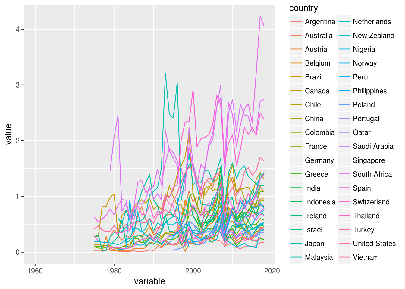
#######################look at overvalued country#######################
mkt_cap_gdp_max_long = melt(subset(mkt_cap_gdp,all_time_high == 1), id = c("country"))
mkt_cap_gdp_max_long$variable = as.numeric(as.vector(mkt_cap_gdp_max_long$variable))
## Warning: NAs introduced by coercion#All the countries
ggplot(data = mkt_cap_gdp_max_long,
aes(x = variable, y = value, colour = country)) +
geom_line()## Warning: Removed 150 rows containing missing values (geom_path).