Does sector rotation - momentum strategy work?
Faber sector rotation strategy is touted as a superior Tactical Asset Allocation strategy that could generate positive Alpha. This is evident in the post here http://stockcharts.com/school/doku.php?id=chart_school:trading_strategies:sector_rotation_roc.
The strategy is pretty simple. Here is how it works,
- First, you choose 9 sectors
- Second, compute the 6 month returns
- Third, you only ‘trade’ once a month. For simiplicity I choose end of the month
- Fourth, you invest in 3 sectors with the highest past 6 month returns. If SnP 500 falls below its 200 day moving average, you do not invest at all.
I was really interested to adopt this strategy! But my hopes were crushed when I did my independent investigation. The returns were bad. And that’s even before adding in commission fees!
I’m unsure why - but I can’t seem to replicate the performance in various articles and the original academic paper.
There may be some careless mistakes in my computation. But allow me to lay out my full analysis.
Updates: There’re indeed careless mistakes; will update the analysis and assess the performance in a more robust manner.
Setting up the analysis by loading in packages and downloading data
I first download 9 sectors’ + Snp 500 worth of data
#Looking into Faber Investment Strategy

library(quantmod)
## Loading required package: xts## Loading required package: zoo##
## Attaching package: 'zoo'## The following objects are masked from 'package:base':
##
## as.Date, as.Date.numeric## Loading required package: TTR## Version 0.4-0 included new data defaults. See ?getSymbols.library(TTR)
## ------------------------------------------------------------------------
symbols = c("XLF", "XLP", "XLE", "XLY", "XLV", "XLI", "XLB", "XLK", "XLU")
startDate <- '1998-01-01'
endDate <- '2018-04-03'
getSymbols(symbols, src='yahoo', index.class=c("POSIXt","POSIXct"), from=startDate, to=endDate, adjust=T)## 'getSymbols' currently uses auto.assign=TRUE by default, but will
## use auto.assign=FALSE in 0.5-0. You will still be able to use
## 'loadSymbols' to automatically load data. getOption("getSymbols.env")
## and getOption("getSymbols.auto.assign") will still be checked for
## alternate defaults.
##
## This message is shown once per session and may be disabled by setting
## options("getSymbols.warning4.0"=FALSE). See ?getSymbols for details.##
## WARNING: There have been significant changes to Yahoo Finance data.
## Please see the Warning section of '?getSymbols.yahoo' for details.
##
## This message is shown once per session and may be disabled by setting
## options("getSymbols.yahoo.warning"=FALSE).## pausing 1 second between requests for more than 5 symbols
## pausing 1 second between requests for more than 5 symbols
## pausing 1 second between requests for more than 5 symbols
## pausing 1 second between requests for more than 5 symbols
## pausing 1 second between requests for more than 5 symbols## [1] "XLF" "XLP" "XLE" "XLY" "XLV" "XLI" "XLB" "XLK" "XLU"dat = merge(XLF[,6],XLP[,6],XLE[,6],XLY[,6],XLV[,6],XLI[,6],XLB[,6],XLK[,6],XLU[,6])
names(dat) = c("XLF", "XLP", "XLE", "XLY", "XLV", "XLI", "XLB", "XLK", "XLU")
getSymbols("^GSPC", src='yahoo', index.class=c("POSIXt","POSIXct"), from=startDate, to=endDate, adjust=T)## [1] "GSPC"GSPC = GSPC[,6]Pre-processing data
Here’s the workhorse of the program. I find the daily 6-month price change and also noted the monthly rebalancing index.
For each day, I also looked at the 3 highest 6 month price-change so that on the end of the month rebalancing, I could easily pick these 3 sectors and place it in my simulation.
GSPC$MA = SMA(GSPC[,1],200)
GSPC$more_MA = ifelse(GSPC[,1] > GSPC$MA,1,0)

#Lag all series by 6 months
lag_dat = dat
for(i in 1:ncol(dat)){
  lag_dat[,i] = Lag(dat[,i],252/2)
}


#And find the price change over 6 months
price_change = (dat - lag_dat)/lag_dat

#Rate of returns
ret = ROC(dat)

#Denote if this month is a rebalancing month
rebal_index = data.frame(index = endpoints(dat,on="months")[-1])

#If yes, pick the 3 stocks-->Use DSI code to pick the highest returns column
#Function for positions of minimum and maximum
maxn <- function(n) function(x) order(x, decreasing = TRUE)[n]
minn <- function(n) function(x) order(x, decreasing = FALSE)[n]

#Super-imposed in column the return for that 3 stocks till next re-bal date
max_index = data.frame(max_1 = apply(price_change,1,maxn(1)),
                       max_2 = apply(price_change,1,maxn(2)),
                       max_3 = apply(price_change,1,maxn(3)))

# max_index[1:(252/2),] = NA
max_index[1:(200),] = NA

#add in 200 day-MA as filter-->Could be an option at the end to change all return values to 0

#Construct a data frame for portfolio simulation
portfolio_sim = dat

portfolio_sim$rebal = 0
portfolio_sim$rebal[1] = 1
portfolio_sim$rebal[2] = 1
# portfolio_sim$rebal[252/2 + 1] = 1
portfolio_sim$rebal[200 + 1] = 1

for(i in 1:nrow(rebal_index)){
  portfolio_sim$rebal[rebal_index$index[i]] = 1
}

#Portfolio simulation
portfolio_sim$max1_ticker = NA
portfolio_sim$max2_ticker = NA
portfolio_sim$max3_ticker = NA

portfolio_sim$max1_ret = 0
portfolio_sim$max2_ret = 0
portfolio_sim$max3_ret = 0

# portfolio_sim$max1_portfolio = 0; portfolio_sim$max1_portfolio[252/2] = 100
# portfolio_sim$max2_portfolio = 0; portfolio_sim$max2_portfolio[252/2] = 100
# portfolio_sim$max3_portfolio = 0; portfolio_sim$max3_portfolio[252/2] = 100
# portfolio_sim$tot_portfolio = 0; portfolio_sim$tot_portfolio[252/2] = 300

portfolio_sim$max1_portfolio = 0; portfolio_sim$max1_portfolio[200] = 100
portfolio_sim$max2_portfolio = 0; portfolio_sim$max2_portfolio[200] = 100
portfolio_sim$max3_portfolio = 0; portfolio_sim$max3_portfolio[200] = 100
portfolio_sim$tot_portfolio = 0; portfolio_sim$tot_portfolio[200] = 300
Start simulation
Moment of truth…I started my simulation - Picking 3 sectors with highest momentum; stick to it for the month. Rinse and repeat this process monthly.
If SnP 500 dips below the 200 day average, I will liquidate any position for the month.
# start = 252/2 + 1
start = 200+ 1
for(i in start:nrow(portfolio_sim)){

  if(as.numeric(portfolio_sim$rebal[i]) == 1){

    #Include the ticker index
    portfolio_sim$max1_ticker[i] = max_index$max_1[i]
    portfolio_sim$max2_ticker[i] = max_index$max_2[i]
    portfolio_sim$max3_ticker[i] = max_index$max_3[i]

    #Include the returns
    portfolio_sim$max1_ret[i] = ret[i,portfolio_sim$max1_ticker[i]]
    portfolio_sim$max2_ret[i] = ret[i,portfolio_sim$max2_ticker[i]]
    portfolio_sim$max3_ret[i] = ret[i,portfolio_sim$max3_ticker[i]]

    #Calculate the portfolio
    portfolio_sim$max1_portfolio[i] = portfolio_sim$tot_portfolio[i-1]/3
    portfolio_sim$max2_portfolio[i] = portfolio_sim$tot_portfolio[i-1]/3
    portfolio_sim$max3_portfolio[i] = portfolio_sim$tot_portfolio[i-1]/3
    portfolio_sim$tot_portfolio[i] = portfolio_sim$max1_portfolio[i] + portfolio_sim$max2_portfolio[i] + portfolio_sim$max3_portfolio[i]

    #if less than 200 day-MA, change max1_ticker to 999
    if(as.numeric(GSPC$more_MA[i]) == 0){
      portfolio_sim$max1_ticker[i] = 999
      portfolio_sim$max2_ticker[i] = 999
      portfolio_sim$max3_ticker[i] = 999
    }

    # print(portfolio_sim$tot_portfolio[i])

  }else{
    portfolio_sim$max1_ticker[i] = portfolio_sim$max1_ticker[i-1]
    portfolio_sim$max2_ticker[i] = portfolio_sim$max2_ticker[i-1]
    portfolio_sim$max3_ticker[i] = portfolio_sim$max3_ticker[i-1]

    #if ticker == 999-->change returns to 0, else use the normal returns
    if(as.numeric(portfolio_sim$max1_ticker[i]) == 999){
      portfolio_sim$max1_ret[i] = 0
      portfolio_sim$max2_ret[i] = 0
      portfolio_sim$max3_ret[i] = 0
    }else{
      #Include the returns based on above index
      portfolio_sim$max1_ret[i] = ret[i,portfolio_sim$max1_ticker[i]]
      portfolio_sim$max2_ret[i] = ret[i,portfolio_sim$max2_ticker[i]]
      portfolio_sim$max3_ret[i] = ret[i,portfolio_sim$max3_ticker[i]]
    }

    #Calculate the portfolio
    portfolio_sim$max1_portfolio[i] = as.numeric(portfolio_sim$max1_portfolio[i-1]) * (1+portfolio_sim$max1_ret[i])
    portfolio_sim$max2_portfolio[i] = as.numeric(portfolio_sim$max2_portfolio[i-1]) * (1+portfolio_sim$max2_ret[i])
    portfolio_sim$max3_portfolio[i] = as.numeric(portfolio_sim$max3_portfolio[i-1]) * (1+portfolio_sim$max3_ret[i])

    portfolio_sim$tot_portfolio[i] = portfolio_sim$max1_portfolio[i] + portfolio_sim$max2_portfolio[i] + portfolio_sim$max3_portfolio[i]
  }

}
Performance analysis
Presto! The performance is real bad. Just by looking at the equity curve, I don’t think there’s any incentive to do further performance anlaysis.
#############################################Carry out performance metrics#############################################
#Subset out NAs
portfolio_sim = subset(portfolio_sim,!is.na(portfolio_sim$max1_ticker))
plot(portfolio_sim$tot_portfolio)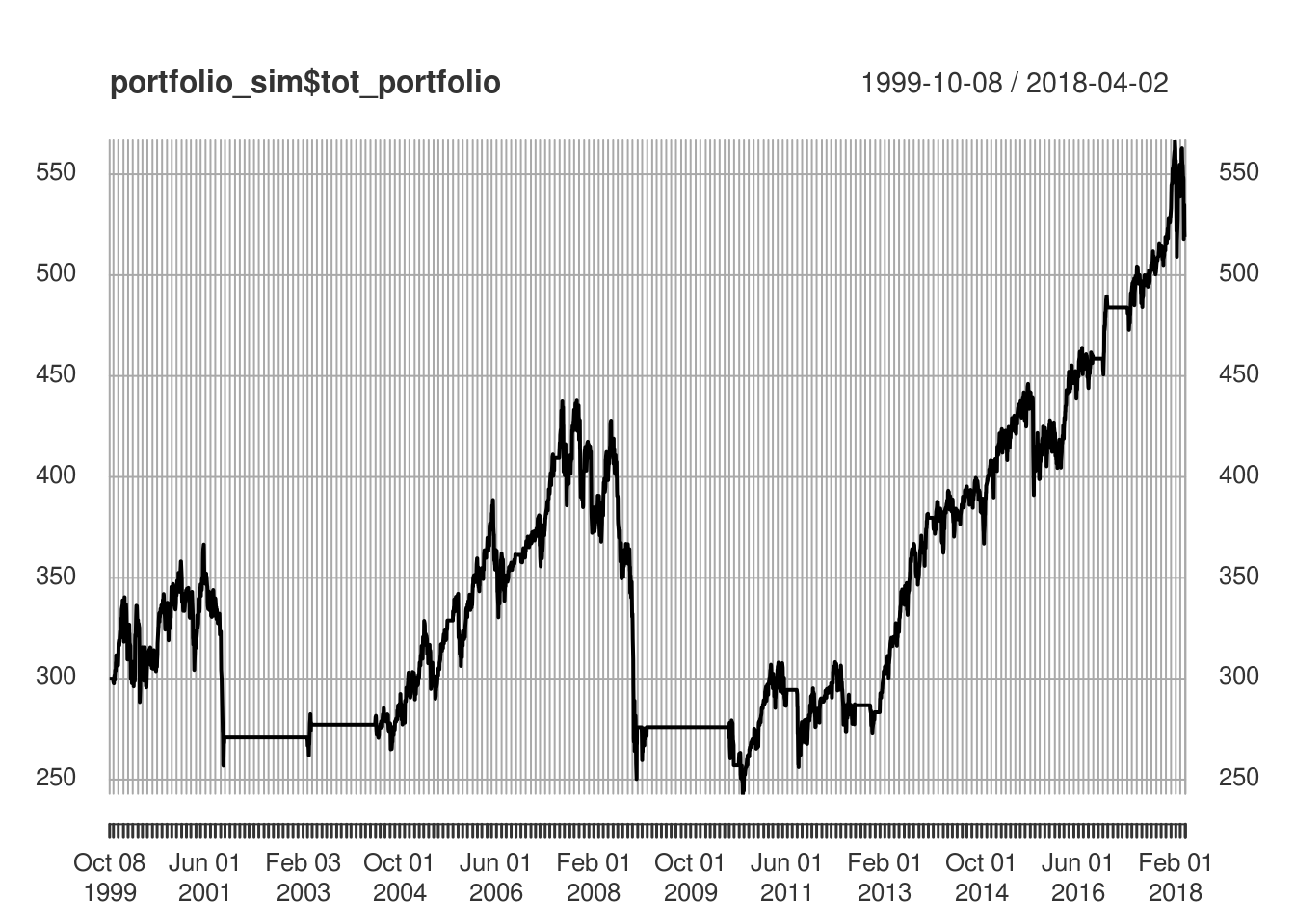
#Find ROC returns