Volatility targeting
Currently, I’ve a suite of toolkits integrated into my Jarvis that advises me on the investing decisions that I’ve to make on a daily basis.
On the latest feature I cobbled together on a Saturday evening, 2 weeks ago, I’ve decided to measure the volatility of my portfolio formally.
Why I’m doing this is because managing risks in the form of volatility is easier than targeting returns.
On any given day, it’s easier to predict volatility than returns itself because of its persistent nature.
Think of it as a coin flips with Binomal distribution: B ~ (n, p).
P is the probability for which you expect a positive expected payout.
And variance of this win-lose distribution is n * p * (1-p). This variance is easier to ‘predict’ based on your win rates.
But market is not simply a binomial distribution, it also needs to take into consideration the portfolio size exposed to market risks and sequence of returns (autocorrelation here) at any given day.
Current distribution of my portfolio win rate is around 65 to 70%. But because of some negative skew in returns, my portfolio is languishing at status quo (0%) since start of the year.
Though my portfolio have outperformed the indexes by a factor of 2 to 3, the steep drawdown during March period of my portfolio could have been prevented if I’ve put a hedge early on (if I’ve done it through a systematic quant way) to maintain a fixed volatility target.
Hence, I decided to integrate the volatility targeting feature into Jarvis that advises me daily on the amount of index hedge to place to maintain my portfolio at a constant volatility target; not a perfect way to maintain volatility target (since my portfolio is not perfectly correlated to index) but I find it cumbersome and potentially costly to sell off multiple counters on a daily basis. I used a global etf as a proxy to maintain my risk level since my portfolio has a global tilt.
Here is the volatility of my levered portfolio. Notice how it spiked up 5 times in the month of March this year.
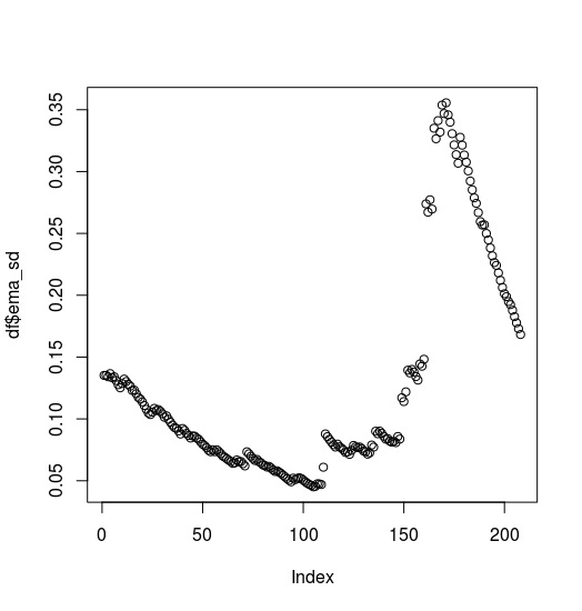
What volatility targeting does is to supposedly to turn the volatility curve into a straight line.
You may find the code below. I won’t delve into the details but this is essentially what it does,
- Obtain my current positions from googlesheet
- Compute my portfolio value converted into SGD now and historically based on current positions
- Compute annual standard deviation (normal and exponential version shared by Robert Carver) of my portfolio based on past 36 days daily returns. Annual non exponential standard deviation returns of portfolio = Daily standard deviation of returns of portfolio * sqrt(252)
- Compute benchmark (VT) volatility
- Compute ‘imperfect’ hedge required to achieve volatility target of 15%
- Pushes a notification to me on how much additional/ lesser hedge is required
#Note: Volatility targeting

#Initialization
sapply(c("ggplot2", "plotly", "quantmod", "pushoverr", "zoo", "dplyr", "roll", "PerformanceAnalytics", "pushoverr", "googlesheets", "pracma", "timeDate", "riingo"), require, character.only = T)
source('util/extract_stock_prices.R')

rsd_file = Sys.getenv("GOOGLESHEET")
gs_auth(token = rsd_file)
suppressMessages(gs_auth(token = rsd_file, verbose = FALSE))

dat = gs_title("Investment")
gs_ws_ls(dat)   #tab names
data <- gs_read(ss=dat, ws = "debt_to_equity", skip=0)
leverage = 1 + data$Ratio[3]
# leverage = 1
current_hedge_value = data$Ratio[nrow(data)]

currency = "SGD=X"
last_date = Sys.Date() - 200
benchmark = "VT"
num_counters = 24

##########################Obtain portfolio info##########################
# df_tickers = data.frame(tickers = c("TLT", "IEF", "SPY", ))
df_tickers <- gs_read(ss=dat, ws = "investment_live", skip=0)
# df_tickers = subset(df_tickers, df_tickers$Ticker != "CNYB.AS")
df_tickers = filter(df_tickers, num_units > 0)

current_value = sum(df_tickers$value)

df_tickers = df_tickers[, 1:5]
df_tickers[which(df_tickers$exch_rate_type == "SGDHKD=X"), 5] = "HKDSGD=X"

##########################Format data function##########################
#Create a time series of data, then merge in. Just filter out weekend only
data_format = function(ticker, num_units, currency, last_date){

  #Create date range
  create_date = function(i){
    return(last_date + i)
  }

  df = data.frame(Date = sapply(0:(Sys.Date() - last_date), create_date))
  df$Date = as.Date(df$Date, origin = "1970-01-1")
  df$isWeekend = isWeekend(df$Date)
  df$Date = as.character(df$Date)

  #Read data
  data_temp = df_crawl_time_series(ticker, "1970-07-01", "2030-12-30")
  data_temp = subset(data_temp, data_temp$Date >= last_date & data_temp$Date <= Sys.Date())
  data = merge(df, data_temp, by = c("Date"), all.x = T)

  #Fill NAs
  data = subset(data, data$isWeekend == F)

  if(is.na(data$Adj.Close[1])){
    data$Adj.Close[1] = data$Adj.Close[2]
  }

  if(is.na(data$Adj.Close[1])){
    data$Adj.Close[1] = data$Adj.Close[3]
  }

  if(is.na(data$Adj.Close[1])){
    data$Adj.Close[1] = data$Adj.Close[4]
  }


  data$Adj.Close = na.locf(data$Adj.Close)

  #Subset out data-frame
  df = data.frame(Date = data$Date, Price = data$Adj.Close, stringsAsFactors = F)

  #Read in num_units
  df$num_units = num_units

  #Subset date range
  df = subset(df, df$Date >= last_date & df$Date <= Sys.Date())

  #Read in currency
  currency = df_crawl_time_series(currency, "1970-07-01", "2030-12-30")
  currency$Adj.Close = na.locf(currency$Adj.Close)
  currency = subset(currency, select = c("Date", "Adj.Close"))

  #Merge in currency
  df = df %>%
    left_join(., currency, by = c("Date"))

  #Convert to local currency
  df$local_unit_value = df$Price * df$Adj.Close
  df$local_value = df$local_unit_value * df$num_units

  #Return date, portfolio value
  df$Date = as.Date(df$Date)

  #ticker
  df$ticker = ticker

  df_sub = subset(df, df$Date >= last_date & df$Date <= Sys.Date())

  return(df_sub)
}

########################Formatting portfolio function####################
portfolio_format = function(df_tickers, last_date){

i = 1
ticker_agg = data_format(df_tickers$Ticker[i], df_tickers$num_units[i], df_tickers$exch_rate_type[i], last_date)

for(i in 2:nrow(df_tickers)){
  print(i)
  ticker_ind = data_format(df_tickers$Ticker[i], df_tickers$num_units[i], df_tickers$exch_rate_type[i], last_date)
  ticker_agg = rbind(ticker_agg, ticker_ind)
}

portfolio = ticker_agg %>%
  group_by(Date) %>%
  summarize(portfolio_value = sum(local_value, na.rm = T),
            num_counters = n()
  )

portfolio$portfolio_value_adj = ifelse(portfolio$num_counters < num_counters, NA, portfolio$portfolio_value)

portfolio$upper_sd = mean(portfolio$portfolio_value_adj, na.rm = T) + 0.4 * sd(portfolio$portfolio_value_adj, na.rm = T)
portfolio$lower_sd = mean(portfolio$portfolio_value_adj, na.rm = T) - 0.4 * sd(portfolio$portfolio_value_adj, na.rm = T)
portfolio$portfolio_value_adj2 = ifelse((portfolio$portfolio_value_adj  > portfolio$upper_sd) | (portfolio$portfolio_value_adj  < portfolio$lower_sd),
                                        NA,
                                        portfolio$portfolio_value_adj)
portfolio$portfolio_value_adj2 = na.locf(portfolio$portfolio_value_adj2)

if(!is.na(current_value)){
  portfolio$portfolio_value_adj2[nrow(portfolio)] = current_value
}

portfolio$returns = ROC(portfolio$portfolio_value_adj2) * leverage
portfolio$returns_100 = portfolio$returns * 100

portfolio$roll_std = roll_sd(portfolio$returns, 36)
portfolio$roll_std_annual = portfolio$roll_std * (252 ^ 0.5)

df = portfolio

return(df)

}

##########################Find beta of portfolio######################################
#Find out how much of local_unit_value needed
find_beta = function(df, benchmark){

  price_bench = data_format(benchmark, num_units = 10, currency, last_date)
  price_bench$returns = ROC(price_bench$local_value)
  price_bench = subset(price_bench, select = c("Date", "returns", "local_unit_value"))
  names(price_bench)[2] = "returns_benchmark"

  df_agg = df %>%
    left_join(., price_bench, by = "Date")

  reg = lm(df_agg$returns ~ df_agg$returns_benchmark)
  return(as.numeric(reg$coefficients[2]))

}

##########################Pure vol targeting######################################
#Find out how much of local_unit_value needed
#Account for leveraged %

find_vol_units = function(df, benchmark, leverage){

  price_bench = data_format(benchmark, num_units=10, currency, last_date)
  price_bench$returns = ROC(price_bench$local_value)
  price_bench = subset(price_bench, select = c("Date", "returns", "local_unit_value"))
  names(price_bench)[2] = "returns_benchmark"

  df_agg = df %>%
              left_join(., price_bench, by = "Date")

  #Compute EMA of VT price. Loop number of units. And iteratively compute new portfolio value and EMA of SD. Find out closest number of VT units required.
  df_agg$square_returns_target = df_agg$returns_benchmark ^ 2
  df_agg$square_returns_target[1] = df_agg$square_returns_target[2]
  df_agg$ema_vol_target =  movavg(df_agg$square_returns_target, 36, type = "e")
  df_agg$ema_sd_target = df_agg$ema_vol_target ^ 0.5 * (252 ^ 0.5)

  df_agg$square_returns = (df_agg$returns) ^ 2
  df_agg$square_returns[1] = df_agg$square_returns[2]
  df_agg$ema_vol =  movavg(df_agg$square_returns, 36, type = "e")
  df_agg$ema_sd = df_agg$ema_vol ^ 0.5 * (252 ^ 0.5)


  return(df_agg)
}

##########################Generate df######################################
df = portfolio_format(df_tickers, last_date)
beta = find_beta(df, benchmark)
df = find_vol_units(df, benchmark, leverage)
reduce_times_exp = df$ema_sd[nrow(df) - 0]/ 0.15

##########################Find hedge required to target risk######################################
hedge = (df$portfolio_value_adj2[nrow(df)] - (df$portfolio_value_adj2[nrow(df)]/ reduce_times_exp)) * (df$ema_sd[nrow(df)] / df$ema_sd_target[nrow(df)])
hedge = round(hedge, 0)

##########################Pushing notifications to inform how much hedge is required######################################
msg = paste0("You should hedge ", hedge,
             " Current hedge value is ", current_hedge_value,
             " Additional hedge required ", (hedge - current_hedge_value),
             " Portfolio vol is ", round(df$ema_sd[nrow(df)], 3),
             " Benchmark vol is ", round(df$ema_sd_target[nrow(df)], 3)
)

print(msg)
plot(df$ema_sd)

if(abs(hedge - current_hedge_value) > 3000){
  pushover(message = msg,
           user = Sys.getenv("pushover_user"), app = Sys.getenv("pushover_app"))

}