Market neutral strategy
As the negative news pile up (trade wars, slump in economy growths, etc), I sought for market neutral stategies that could perform well in any market environment.
An idea that struck me recently is to exploit the pair between Berkshire and SnP 500 ETF.
The SnP500 ETF/ Berkshire ratio has been falling over the years - insinuating that Berkshire still outperforms the index in the last couple of years.
And what’s more impressive, it’s still widely regarded as a safe haven in times of trouble.
Strategy
As the market is facing headwind and I sought for a market neutral strategy.
Here’s what I did,
- I derive the SnP500 ETF/ Berkshire ratio over last 5 years
- And I fix a Bollinger Band around the ratio with n = 200 days as the moving average parameter - with 2 SD as the lower (lb) and upper bound (ub) line. Bollinger band ratio accounts for the downward trend in the ratio over time.
- If the ratio is below the lb, I will long SnP500 and short Berkshire Hathaway. And when it mean reverts and touches the middle moving average, I will exit the positions
- Conversely if the ratio is above the ub, I will short SnP500 and long Berkshire Hathaway. Similarly, I will exit the position when it touches the moving average
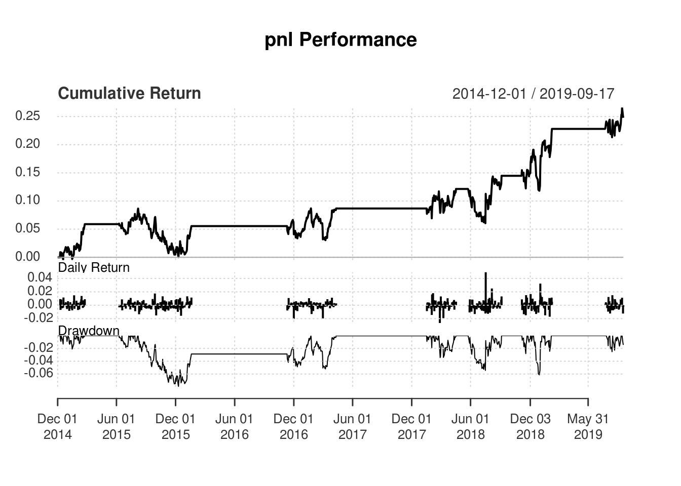
Results
So how did the strategy fare? Fairly impressive I must say.
Sharpe ratio is around 0.65. Annualized return is around 4.5% with the positions only in the market 30% of the time!
That being said, I’m cherry picking here because the performance before this period is sub-par; probably because of a change in market regime. You may execute my code to stress-test this simple strategy.
Disclosure
- I executed a long (BRK-B) short (SPY) strategy on 26-August with approximately $11500 on both positions. Cash outlay is only 11500 dollars on long side. I’m also earning further 2% interest on cash received from short sale held as collateral. I entered at a ratio of 1.439 with expected profits of 5-6% excluding further 2% p.a. of interest on short sale cash.
- Max holding period is 27 work days based on half life formula here (http://en.wikipedia.org/wiki/Ornstein-Uhlenbeck_process) as advised by Ernest Chan. See his example for further explanation
- I’m using pushoverr notification api linked to my phone app within my cron task scheduler. It will inform me to close my positions when the ratio dips below moving average.
Running packages
##                  zoo                tidyr                 plyr
##                 TRUE                 TRUE                 TRUE
##                dplyr               gtools         googlesheets
##                 TRUE                 TRUE                 TRUE
##             quantmod                 urca PerformanceAnalytics
##                 TRUE                 TRUE                 TRUE
##             parallel                  TTR
##                 TRUE                 TRUE
Function
#Function using bollinger band
lf_bollinger_pair_trading = function(stock1, stock2, start_date, end_date, prop_res, bband_days){

#Start of function
data1 = df_crawl_time_series(stock1, start_date, end_date)
data1 = base::subset(data1, select = c("Date", "Open", "Adj.Close"))
names(data1) = c("Date", "Open", "Close")
data1$Date = as.Date(data1$Date)

data2 = df_crawl_time_series(stock2, start_date, end_date)
data2 = base::subset(data2, select = c("Date", "Open", "Adj.Close"))
names(data2) = c("Date", "Open", "Close")
data2$Date = as.Date(data2$Date)

#Training and testing index
data1 = xts(data1[, -1], order.by = data1[, 1])
data2 = xts(data2[, -1], order.by = data2[, 1])

data = merge(data1, data2)
data = as.data.frame(data)
data = subset(data, !is.na(data$Close) & !is.na(data$Close.1))

data$ratio = data$Close/ data$Close.1

# plot(data$ratio)
bb_ratio = data.frame(BBands( data$ratio, n = bband_days))
data = cbind(data, bb_ratio)
data_sub = tail(data, round(nrow(data) * prop_res, 0))

plot(data_sub$ratio)
lines(data_sub$mavg, col = "red")
lines(data_sub$up, col = "blue")
lines(data_sub$dn, col = "green")

#If lower than
data_sub$longs <- data_sub$ratio <= data_sub$dn # buy spread when its value drops below 2 standard deviations.
data_sub$shorts <- data_sub$ratio >= data_sub$up # short spread when its value rises above 2 standard deviations.

#  exit any spread position when its value is at moving average
data_sub$longExits   <- data_sub$ratio >= data_sub$mavg
data_sub$shortExits <- data_sub$ratio <= data_sub$mavg


# #  define indices for training and test sets
# trainset <- 1:as.integer(nrow(data) * prop_train)
# testset <- (length(trainset)+1):nrow(data)

#Signal
data_sub$posL1 = NA
data_sub$posL2 = NA
data_sub$posS1 = NA
data_sub$posS2 = NA

# initialize to 0
data_sub$posL1[1] <- 0; data_sub$posL2[1] <- 0
data_sub$posS1[1] <- 0; data_sub$posS2[1] <- 0

data_sub$posL1[data_sub$longs] <- 1
data_sub$posL2[data_sub$longs] <- -1

data_sub$posS1[data_sub$shorts] <- -1
data_sub$posS2[data_sub$shorts] <- 1

data_sub$posL1[data_sub$longExits] <- 0
data_sub$posL2[data_sub$longExits] <- 0
data_sub$posS1[data_sub$shortExits] <- 0
data_sub$posS2[data_sub$shortExits] <- 0

#positions
data_sub$posL1 <- zoo::na.locf(data_sub$posL1); data_sub$posL2 <- zoo::na.locf(data_sub$posL2)
data_sub$posS1 <- zoo::na.locf(data_sub$posS1); data_sub$posS2 <- zoo::na.locf(data_sub$posS2)
data_sub$position1 <- data_sub$posL1 + data_sub$posS1
data_sub$position2 <- data_sub$posL2 + data_sub$posS2

#Returns
data_sub$dailyret1 <- ROC(data_sub$Close) #  last row is [385,] -0.0122636689 -0.0140365802
data_sub$dailyret2 <- ROC(data_sub$Close.1) #  last row is [385,] -0.0122636689 -0.0140365802

#Backshifting here. But signal is for following day returns!. So can still use latest Z-score
data_sub$date = as.Date(row.names(data_sub))
data_sub = xts(data_sub[,-which(names(data_sub) == "date")], order.by = data_sub[, which(names(data_sub) == "date")])

#Doesn't account for number of shares!!!!!
data_sub$pnl = lag(data_sub$position1, 1) * data_sub$dailyret1  + lag(data_sub$position2, 1) * data_sub$dailyret2

#Performance analytics
tryCatch({
  # charts_perf = charts.PerformanceSummary(data_sub$pnl)
  charts.PerformanceSummary(data_sub$pnl)
}, error = function(e){})

dd = table.Drawdowns(data_sub$pnl)
ds_risk = table.DownsideRisk(data_sub$pnl)
ret = table.AnnualizedReturns(data_sub$pnl)


df_ret = list(data_sub = data_sub,
              dd = dd,
              ds_risk = ds_risk,
              ret = ret
              )

return(df_ret)

}
#Parameters to be includded in function
stock1 = "SPY"
stock2 = "BRK-B"
start_date = "2000-07-01"
end_date = "2019-12-30"
prop_res = 0.25 #Proportion of results to show
bband_days = 200 #Bollinger band of ratio
#Storing result to function
res = lf_bollinger_pair_trading(stock1, stock2, start_date, end_date, prop_res, bband_days)## 'getSymbols' currently uses auto.assign=TRUE by default, but will
## use auto.assign=FALSE in 0.5-0. You will still be able to use
## 'loadSymbols' to automatically load data. getOption("getSymbols.env")
## and getOption("getSymbols.auto.assign") will still be checked for
## alternate defaults.
##
## This message is shown once per session and may be disabled by setting
## options("getSymbols.warning4.0"=FALSE). See ?getSymbols for details.##
## WARNING: There have been significant changes to Yahoo Finance data.
## Please see the Warning section of '?getSymbols.yahoo' for details.
##
## This message is shown once per session and may be disabled by setting
## options("getSymbols.yahoo.warning"=FALSE).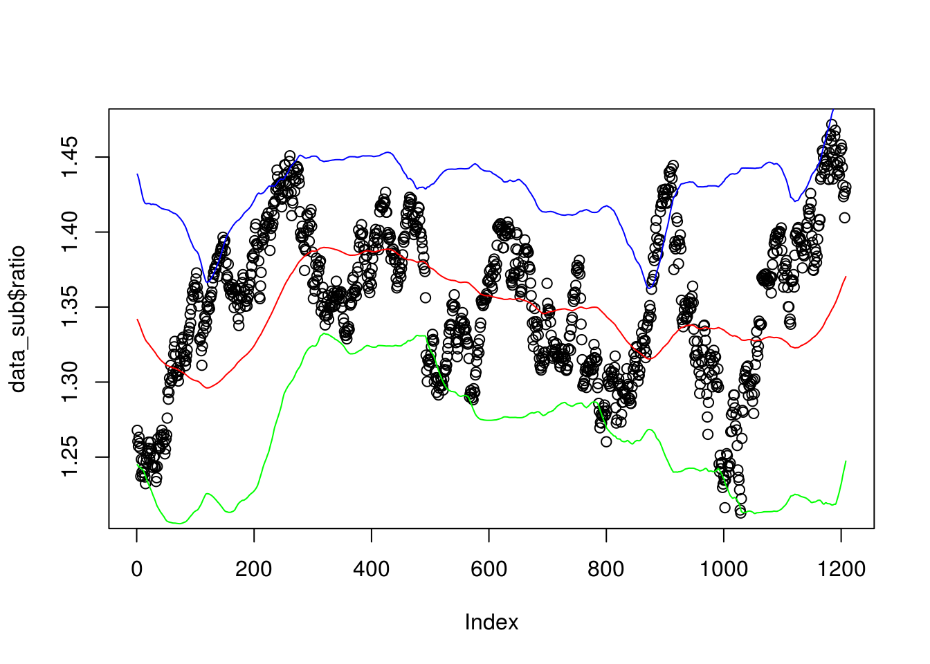
Displaying of results
- Drawdown period
res$dd## From Trough To Depth Length To Trough Recovery
## 1 2015-08-10 2015-12-10 2017-01-23 -0.0793 367 87 280
## 2 2018-12-13 2018-12-31 2019-01-08 -0.0612 17 12 5
## 3 2018-05-25 2018-07-17 2018-08-06 -0.0543 50 36 14
## 4 2017-01-24 2017-03-09 2018-01-26 -0.0520 255 32 223
## 5 2018-02-26 2018-02-27 2018-04-11 -0.0343 32 2 30- Downside risk
res$ds_risk## pnl
## Semi Deviation 0.0030
## Gain Deviation 0.0050
## Loss Deviation 0.0041
## Downside Deviation (MAR=210%) 0.0092
## Downside Deviation (Rf=0%) 0.0029
## Downside Deviation (0%) 0.0029
## Maximum Drawdown 0.0793
## Historical VaR (95%) -0.0066
## Historical ES (95%) -0.0106
## Modified VaR (95%) -0.0039
## Modified ES (95%) -0.0039- Returns
res$ret## pnl
## Annualized Return 0.0473
## Annualized Std Dev 0.0717
## Annualized Sharpe (Rf=0%) 0.6601